Virtualize your multi-head microscope

Syncing viewports across different users

Ever wanted to be able to have one user at the driver’s seat while others are watching, each looking at their own screen, just like with multi-head microscopes but over the internet? This can probably be accomplished with a screen sharing & conferencing tool, but the image quality results may be poor. How about allowing all users to take over the viewport at the same time? Drawing annotations simultaneously? Allowing users to share multiple viewports? Have this functionality in your application? It gets more complicated now, right? Wrong.

PMA.live enables exactly this functionality out of the box and can be integrated in your application without a lot of coding or complicated setup procedures. How does it work and why is it more efficient than your traditional screen share? Because PMA.live tells connected clients which tiles to download, and each client then retrieves said tiles directly from the tile server. This is more efficient and elegant than to broadcast pixels.

The ingredients you need are:

  • PMA.core – Where digital slides come from
  • PMA.UI – the UI Javascript library
  • PMA.live – Pathomation’s collaboration platform

In the page where we want to add collaboration functionality we need the following JS libraries included:

Let’s start by syncing a single viewport. In the PMA.live terminology, enabling users to collaborate with each other by looking at the same slides is called a session. Therefore, a user must first create a session which the rest of the participants have to join.

The first step is to establish a connection to the PMA.live backend:

Collaboration.initialize(
{
	pmaCoreUrl: pmaCoreUrl,
	apiUrl: `${collaborationUrl}api/`,
	hubUrl: `${collaborationUrl}signalr`,
	master: isMaster,
	dataChanged: collaborationDataChanged,
	pointerImageSrc: "pointer.png",
	masterPointerImageSrc: "master-pointer.png",
	getSlideLoader: getSlideLoader,
}, [])

The initialize method tells to the PMA.live Collaboration static object where to find PMA.core, PMA.live backend, whether or not the current user is the session owner, what icons to show for the users’ and the master’s cursor and accepts a couple of callback functions which we will explain later.

Once PMA.live has been initialized, we can continue by either creating or joining a session:

Collaboration.joinSession(sessionName, sessionActive, userNickname, everyoneInControl);

The joinSession method will create a session if it does not exist and then join it. If the session doesn’t exist, it is possible to specify whether or not it is currently active and if all users can take control of the synced viewports or only if the session owner can do this. Once the session has been created, only the session owner can modify it and change it’s active status or give control to others.

In order for PMA.live to be able to sync slides, it has to know the viewports it should work with. In this example, we will first create a slide loader object:

const sl = new PMA.UI.Components.SlideLoader(context, {
				element: slideLoaderElementSelector,
				filename: false,
				barcode: false,
			});

Now let’s tell PMA.live that we are only going to be syncing a single viewport:

Collaboration.setNumberOfImages(1);

Now let’s go back to the implementation of the “getSlideLoader” callback that we used during the initialization of PMA.live. This function will be called by PMA.live when it needs to attach to a viewport in order to control it. So the implementation in this example looks like this:

function getSlideLoader(index, totalNumberOfImages) {
	return sl;
}

We just return the one and only slide loader that we instantiated earlier.

Finally, let’s talk about the “collaborationDataChanged” callback. PMA.live uses SignalR and the WebSocket protocol to achieve real time communication between participants. Besides the out of the box slide syncing capabilities, it gives you the ability to exchange data between the users, in real time. This could be useful for example if you wanted to implement a chat system on top of the session. Every user can change the session’s data by invoking the Collaboration.setApplicationData method. It accepts a single object that will be shared among users. Whenever this method is called, all other users will receive it through the collaborationDataChanged callback, which looks like this:

function collaborationDataChanged() {
	console.log("Collaboration data changed");
	console.log(Collaboration.getApplicationData());
}

Summing it all up, PMA.live provides an easy way to enable real time collaboration between users. It takes away the burden, of syncing data and digital slides, from the developer and allows you to focus on the integration of the Pathomation toolbox in your application.

You can find a complete example of PMA.live here.

What whole slide images (WSIs) are made of

Whole Slide Images

If you already know about pyramidical image files, feel free to skip this paragraph. If you don’t, sticks around; it’s important to understand how microscopy data coming out of slide scanners is structured to be able to manipulate it.

It all starts with a physical slide: a physical slide is a thin piece of glass, with the dimensions

When a physical slide is registered in a digital fashion, it is translated into a 2-dimensional pixel matrix. At a 40X magnification, it takes a grid of4 x 4 pixels to represent 1 square micrometer. We can also say that the image has a resolution of 0.25 microns per pixel. This is also expressed as 4 pixels per micron (PPM).

All of this means that in order to present our 5 cm x 2 cm physical specimen from the first part of this tutorial series in a 40X resolution we need (5 * 10 * 1000 * 4) * (2 * 10 * 1000 * 4) = 200k x 80k = 16B pixels

Now clearly that image is way too big to load in memory all at once, and even with advanced compression techniques, the physical sizes of these is roughly around one gigabyte per slide. So what people have thought of is to package the image data as a pyramidal stack.

Pyramid of Cestius as a metaphore for pyramidal stack images. By Francesco Gasparetti from Senigallia, Italy – Piramide Cestia, CC BY 2.0, https://commons.wikimedia.org/w/index.php?curid=2614848

Ok, perhaps not that kind of pyramid…

But you can imagine a very large image being downsampled a number of times until it receives a manageable size. You just keep dividing the number of pixels by two, and eventually you get a single image that still represents the whole slide, but is only maybe 782 x 312 pixels in size. This then becomes the top of your pyramid and we label it as zoomlevel 0.

At zoomlevel 1, we get a 1562 x 624 pixel image etc. It turns out that our original image of 200k x 80k pixels is found at zoomlevel 8. Projected onto our pyramid, we get something like this:

Worked out example (showing the different zoomlevels) of a pyramidal stack for a concrete whole slide image.

So the physical file representing the slide doesn’t just store the high-resolution image, it stored a pyramidal stack with as many zoomlevels as needed to reach the deepest level (or highest resolution). The idea is that depending on the magnification that you want to represent on the screen, you read data from a different zoomlevel.

Tiles

The pyramid stack works great up to certain resolution. But pretty quick we get into trouble and the images become too big once again to be shown in one pass. And of course, that is eventually what we want to do: Look at the images in their highest possible detail.

In order to work around this problem, the concept of tiles is introduced. The idea is that at each zoomlevel, a grid overlays the image data, arbitrarily breaking the image up in tiles. This leads to a representation like this:

Now, for any area of the slide that we want to display at any given time to the end-user, we can determine the optimal zoomlevel to select from, as well a select number of tiles that are sufficient to show the desired “field of view”, rather than asking the user to wait to download the entire (potentially huge!) image. This goes as follows:

Or, put the other way around (from the browser’s point of view):

So there you have it: whole slide images are nothing but tiled pyramid-shaped stacks of image data.

Building digital pathology web apps with PHP

PHP != Python

Earlier we announced the availability of our PHP API.

It is worth pointing out that not all functionality from the Python API was taken over in the PHP API.

In turn, the PHP API introduces some interesting options weren’t available in the original Python interface, either (and that are probably worth bringing over to our Java API as a result).

Some functionality is (or will be, based on our most recently gained insights) available in all platform. We leave it up to you to determine which one makes the most sense given your habitat.

Here’s an interesting example. In our Python tutorial series, one of the things we do is load a slide’s thumbnail and send it to MatPlotLib’s pyplot.

Translating our Python functionality to PHP, we get:

<?php
include_once "lib_pathomation.php";

Use  Pathomation\PmaPhp\Core;

// connect to PMA.start
$session = Core::connect();

// pick up the first slide available in the C:\my_slides directory
$slides = Core::getSlides("C:/my_slides/", $session);
$my_slide = $slides[0];

// retrieve the slide's thumbnail as a GD image object
$thumb = Core::getThumbnailImage($my_slide);

// output JPEG content to webbrowser
header("Content-Type: image/png");
imagejpeg($thumb);
imagedestroy($thumb);
?>

However, this is a rather futile exercise: we’re sending image content back to the browser. A much easier way is to send back a URL to the browser of where the thumbnail is located. Let the browser figure it out from there; that’s why it exists in the first place.

A more PHP-ish way to render a slide’s thumbnail is:

<?php
 include_once "lib_pathomation.php";

Use  Pathomation\PmaPhp\Core;

// connect to PMA.start
 $session = Core::connect();

// pick up the first slide available in the C:\my_slides directory
 $slides = Core::getSlides("C:/my_slides/", $session);
 $my_slide = $slides[0];

header("location: ".Core::getThumbnailUrl($my_slide));
 ?>

The following syntax then just looks silly:

<img src="showThumbnail.php?slide=<?php echo urlencode($my_slide); ?>" />

Compare this to the following:

<img src="<?php echo Core::getThumbnailUrl($my_slide); ?>" />

Remember Larry Wall: why bother parsing the content of the thumbnail first ourselves, if we can completely delegate this to the webbrowser?

We still take care to provide data in a host environment’s most “naturally” feeling format.

Case in point: in Python we give you image data in PIL(low) format, in PHP we use GD.

The question that you have to ask yourself: does it make sense to work with GD image data yourself, or is it easier and more convenient to refer to a resource by its URL directly?

PHP introduction

Let’s look at some simple PHP-Pathomation interaction code. The following code is pretty much standard for each script you’ll write:

// include the interaction library
include_once "lib_pathomation.php";

// indicate what functionality you want from the library
Use  Pathomation\PmaPhp\Core;

// connect to PMA.start
$session = Core::connect();

Note that when you connect to a commercial version of PMA.core, only the last line of your code needs to change:

$session = Core::connect("http://my_server/my_pma_core", "user", "pass");

More so then in Python, in PHP you have to frequently ask yourself whether an action is taking place on the webserver back-end side or in the webbrowser client.

A good example of this is the isLite() method. Similar to its Python (and Java) counterpart, it checks and verifies PMA.start is found running. This function only is useful when you’re either using the PHP Command-line interface (CLI):

<?php
// load library
require "lib_pathomation.php";
use  Pathomation\PmaPhp\Core;

// test for PMA.core.lite (PMA.start)
echo "Are you running PMA.core.lite? ".(Core::isLite() ? "Yes!": "no :-(");

Alternatively, the method can be used when you’re developing for PMA.start and you’re guaranteed to have server and client operate at the level of the same localhost setup.

Working with slides

The PHP Core class comes with a number of methods to navigate WSI slides on your local hard disk. Most often you’ll be alternating between getDirectories and getSlides.

Here’s a script that will allow you to navigate your hard disk in a tree-like fashion (place this in c:\inetpub\wwwroot of your (localhost) IIS setup):

<?php
require_once "lib_pathomation.php";

use  Pathomation\PmaPhp\Core;

if (!Core::isLite()) {
 die("PMA.start not found");
}

Core::connect();

echo "<ul>";
if (!isset($_GET["p"])) {
 foreach (Core::getRootDirectories() as $rd) {
  echo "<li><a href='?p=".urlencode($rd)."'>$rd</li>";
 }
} else {
 $parts = explode("/", $_GET["p"]);
 foreach (Core::getRootDirectories() as $rd) {
  if ($parts[0] == $rd) {
   echo "<li><b>$rd</b>";
   foreach (Core::getDirectories($rd) as $subdir) {
    echo "<ul>";
    $subdirParts = explode("/", $subdir);
    if (stripos($_GET["p"], $subdir) === 0) {
     echo "<li><b>".end($subdirParts)."</b>";
     // keep drilling down, or see if you can retrieve slides as well     
     echo "</li>";
    } else {
     echo "<li><a href='?p=".urlencode($subdir)."'>".end($subdirParts)."</a></li>";
    }
    echo "</ul>";
   }
   echo "</li>";
  } else {
   echo "<li><a href='?p=".urlencode($rd)."'>$rd</a></li>";
  }
 }
}
echo "</ul>";
?>

Yes, this should all be in a recursive function so you can dig down to just about any level in your tree structure. However, this post is not about recursive programming; we’re mostly interested in showing you what our API/SDK can do.

For instance, you can retrieve the slides in a selected folder and generate a link to them for visualization:

 // now handle the slides in the subfolder
 echo "<ul>";
 foreach (Core::getSlides($subdir) as $slide) {
  $slideParts = explode("/", $slide);
  echo "<li>".end($slideParts)."</li>";
 }
 echo "</ul>";

Introducing the UI class

We can do better than our last example. Providing a link to PMA.start is easy enough, but once you get to that level you’ve lost control over the rest of your layout. What if you make a website where you want to place slides in certain predefined locations and placeholders?

That’s where the UI class comes in. Currently, you can use it to either embed slide viewports, or thumbnail galleries in your own website.

Here’s how you can include an arbitrary slide:

<?php
// load library
include_once "lib_pathomation.php";

Use  Pathomation\PmaPhp\UI;
Use  Pathomation\PmaPhp\Core;

// setup parameters
UI::$_pma_ui_javascript_path = UI::$_pma_start_ui_javascript_path;
$session = Core::connect();

// pick a slide to embed in your page
$slides = Core::getSlides("C:/my_slides/");
$slide = $slides[0];

// actually embed slide
UI::embedSlideBySessionID(Core::$_pma_pmacoreliteURL, $slide, $session);
?>

The embedSlideBySessionID() method return a string that serves as an identifier for the generated viewport. Use this identifier to subsequently define a style for your viewport:

<?php
// actually embed slide
$viewport = UI::embedSlideBySessionID(Core::$_pma_pmacoreliteURL, $slide, $session);
?>
<style type="text/css">
/* viewport style; as defined by PHP */
#<?php echo $viewport; ?> {
 width: 500px;
 height: 500px;
 border: 2px dashed green;
}
</style>

The result is now a 500 x 500 fixed square (with a dashed border) that doesn’t change as your modify the browser window:

You can have as many viewports on a single page as you want; each is automatically assigned a new ID, and so you can set separate layout for each one.

Working with galleries

What if you have a collection of slides and you want to present an overview of these (browsing through slide filenames is tiring and confusing). You could already combine the code we have in this post so far and request thumbnails for a list of a slides found in a directory, subsequently rendering selected slides in a viewport.

But what if you have 50 slides in the folder? Do you really want to handle the scrolling, just-in-time rendering of initially hidden thumbnails etc.?

Pretty early on in our Pathomation career we found ourselves facing the same problems. We re-invented our own wheel a couple of times, after which we figured it was round enough to encapsulate in a piece of re-usable code.

You guessed it: the UI class provides a way to generate galleries, too. At its simplest implementation, only one line of code is needed (setup not included):

<?php
include_once "lib_pathomation.php";

Use  Pathomation\PmaPhp\UI;
Use  Pathomation\PmaPhp\Core;

$session = Core::connect();
echo "<p>".$session."</p>\n";

UI::$_pma_ui_javascript_path = UI::$_pma_start_ui_javascript_path;

UI::embedGalleryBySessionID(Core::$_pma_pmacoreliteURL, "C:/my_slides", $session);
?>

You’ll notice that you can select slides in the gallery, but they’re not particularly reactive. For that, you’ll need to instruct PMA.UI to provide a viewport as well. When a slide is clicked in the gallery, the slide is then shown in the viewport:

UI::linkGalleryToViewport($gallery, "viewer");

The default orientation of a gallery is “horizontal”, but you can set it to a vertical layout, too:

$gallery = UI::embedGalleryBySessionID(Core::$_pma_pmacoreliteURL, "C:/my_slides", $session, array("mode" => "vertical"));

In which you can build something that looks like this:

Try it!

You can build pretty complicated interfaces already this way. One possibly scheme e.g. is where you offer end-users the possibility to compare slides. You need two galleries and two viewports, and that goes like this:

<table width="100%">
<tr>
<th width="50%">Slide 1</th>
<th width="50%">Slide 2</th>
</tr>
<tr>
<td width="50%" valign="top">
 <?php
 $galLeft = UI::embedGalleryBySessionID(Core::$_pma_pmacoreliteURL, "C:/my_slides", $session);
 ?>
</td>
<td width="50%" valign="top">
 <?php
 $galRight = UI::embedGalleryBySessionID(Core::$_pma_pmacoreliteURL, "C:/my_slides", $session);
 ?>
</td>
</tr>
<tr>
<td width="50%" valign="top">
 <?php
 UI::linkGalleryToViewport($galLeft, "viewerLeft");
 ?>
</td>
<td width="50%" valign="top">
 <?php
 UI::linkGalleryToViewport($galRight, "viewerRight");
 ?>
</td>
</tr>
</table>

Under the hood

Everything PHP spits out is HTML, JavaScript, or CSS. Essentially, the only means of communication PHP has is to provide instructions to the webrowser.

The PHP SDK demonstrated in this post do the same thing: simple single-line instructions in PHP are translated in whole parts of JavaScript code. The UI class takes care of loading all the required libraries, and makes sure housekeeping is taken care of in case of multiple viewports, galleries, etc.

You can see this for yourself by looking at the source-code of your PHP page, after it loads in the webbrowser.

The JavaScript framework that we wrote ourselves for browser-based WSI visualization is called PMA.UI. It comes with its own set of tutorials, and there is much more you can do with PMA.UI than through the PHP SDK alone.

However, we found in practice that there is much demand for cursive embedding of WSI content in any number of places on a website or corporate intranet. In my cases, a gallery browser and a “live” slide viewport are sufficient. In those scenarios, the PHP SDK can definitely come in handy and offer a reduced learning curve.

The SDK should help you get started . By studying the interaction between the PHP-code and the generated JavaScript, you can eventually master the PMA.UI library as well and interact with it directly.

By all means, do send us screenshots of your concoctions (let us know when you need help from your friendly neighborhood pathologists, too)! Perhaps we can have a veritable “wall of WSI fame” up one day.

Three’s a charm: availability of Pathomation’s SDK for PHP

Why PHP?

It is not without pride that I’m announcing here the Pathomation SDK for PHP in addition to our earlier SDK releases for Python and Java.

The reason why we decided to add PHP to the mix is that much web-based software is written in PHP, and PHP is just much quicker to get something started in than Java (or Python). PHP is also the first library where we introduce a UI class, which wraps around PMA.UI, our JavaScript framework.

Our SDK therefore now support three environments, each for their own purposes:

  • PHP: web development
  • Java: back-end (J2EE) integration
  • Python: scripting, image analysis

This is not to say that you can’t use Python for web development, or Java for scripting. There’s some overlap, too. If you’re a seasoned PHP developer and you want to generate overnight reports of newly scanned slides, you may not find it worth the hassle to learn Python, just for this one-time task.

The important thing here is that we support all three languages, no matter what your preference is.

We’ve also dabbled a bit in Ruby (thank you Alexandr Kulinich!), but don’t see any concrete need (yet) to come out (and maintain) a formal SDK library for it, Contact us if you think we are wrong about this.

Seamless transitioning

Pathomation’s SDK interacts with both PMA.start as well as our commercial PMA.core offering. This was done to allow for painless transitioning from one environment to the next. If you decide to switch from PMA.startto its bigger brother PMA.core, you don’t have to re-learn anything. Just add authentication credentials when you establish your first PMA.core connection, and you’re good to go.


blur detection in z-stacks

Z-stacking

Tissue presented on a glass slide can be obtained in three fashions: tissue slides by a microtome from a FFPE tissue block is typically completely flat. This means a scanner can usually obtain an optimal focus point and scan a large area of tissue in a single pass.

The two other types of samples however are typically not flat: both cytological samples and needle aspirations contain clumps of cell (a pap smear test is a good example); if samples from FFPE tissue blocks are mirror-like surfaces (at least with respect to smoothness), then cytological samples are more like the gravel surface on a tennis court.

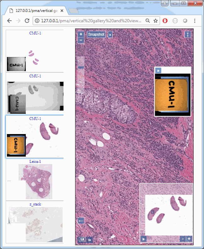
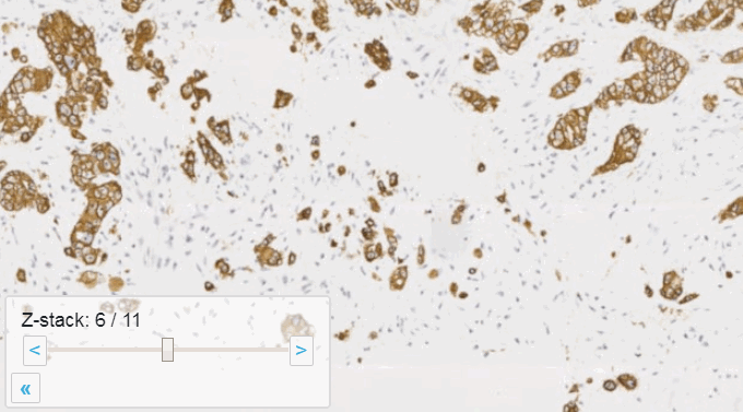
Slide scanners can’t decide on a single layer within the tissue to obtain a “one size fits all” focus, so they typically scan a number of sequential planes. This is your z-stack. Pathomation software supports z-stack data from various scanner vendors.

Beyond viewing

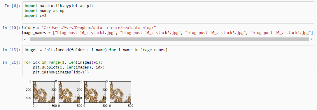
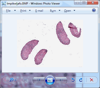
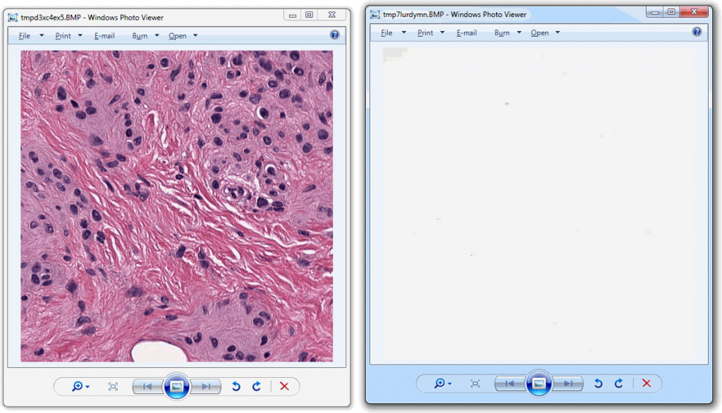
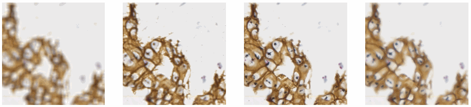
Allowing an end-user to navigate through a z-stack is nice, but can be very tedious and time consuming. Imagine that we have a z-stack with 4 images, then each individual layer can look like this:

A skilled pathologist or researcher can scan through a complete slide in under 10 minutes, but it takes time to acquire this skill, and even so: much of that time is still spent zooming in and out, looking for the optimal sharpness in many regions of the slide.

Can we then use an algorithm to at least select out the most out-of-focus and in-focus tiles in a tiled z-stack? Of course the answer is yes (or we wouldn’t be writing about it)!

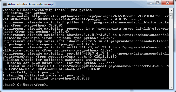
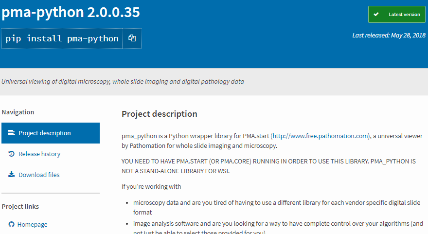
To follow along with the rest of this blog, you’ll need a Jupyter environment (we use Anaconda), a Python programming environment, as well as the PMA_python, Matplotlib, Numpy, and OpenCV packages. You can learn here about setting up PMA_python in Anaconda; take care that you install OpenCV with the correct package name, too (it’s PyPI package name is actually opencv-python, even though you import it into your code as “cv2”):

Let’s first see about reading in all images in an array (and visualize them as a sanity check):

import matplotlib.pyplot as plt
import numpy as np
import cv2

folder = "C:/Users/Yves/blog/"
image_names = ["z-stack1.jpg", "z-stack2.jpg", "z-stack3.jpg", "z-stack4.jpg"]

images = [plt.imread(folder + i_name) for i_name in image_names]

for idx in range(1, len(images)+1):   
    plt.subplot(1, len(images), idx)
    plt.imshow(images[idx-1])

Next, let’s apply an OpenCV blurring filter on each image and compute the difference between the pixel-values in the original image and the blurred image.

blur = []
diff = []

for idx in range(0, len(images)):
    blur.append(cv2.blur(images[idx],(5,5)))
    diff.append(np.abs(blur[idx] - images[idx]))

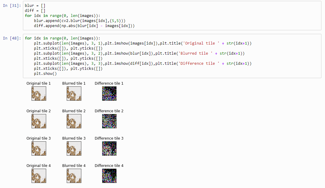
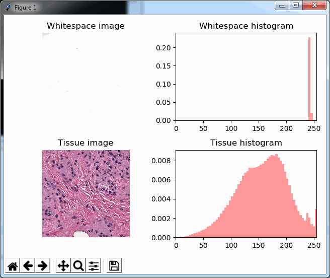
And plot the result (although admittedly visualization of the diff-arrays doesn’t necessarily reveal much information):

for idx in range(0, len(images)):
    plt.subplot(len(images), 3, 1),plt.imshow(images[idx]),plt.title('Original tile ' + str(idx+1))
    plt.xticks([]), plt.yticks([])
    plt.subplot(len(images), 3, 2),plt.imshow(blur[idx]),plt.title('Blurred tile ' + str(idx+1))
    plt.xticks([]), plt.yticks([])
    plt.subplot(len(images), 3, 3),plt.imshow(diff[idx]),plt.title('Difference tile ' + str(idx+1))
    plt.xticks([]), plt.yticks([])
    plt.show()

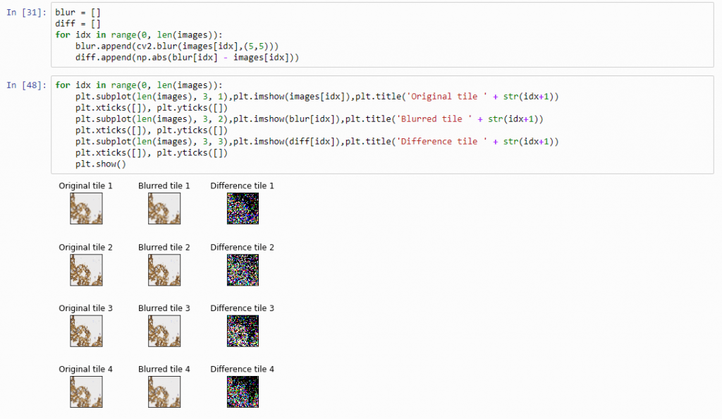
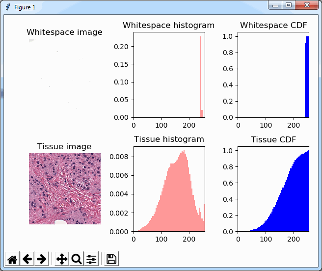
The idea behind our exercise is the following: a blurred image that is blurred, will show less difference in pixel-values, compared to a sharp images that is blurred with the same filter properties.

Therefore, we can now compute the sum of all the values in the diff-array and identify the indices of the lowest and highest values. For our z-stack, the index that contains the smallest summed differences will point to the blurriest (or “most blurred”?) image; the index that contains the largest summed difference will point to the sharpest image. Let’s see if this works:

diff_sums = [np.sum(arr) for arr in diff]

idx_blurriest = diff_values.index(np.min(diff_sums))
idx_sharpest = diff_values.index(np.max(diff_sums))

plt.subplot(121)
plt.imshow(images[idx_blurriest])
plt.title("Blurriest tile")

plt.subplot(122)
plt.imshow(images[idx_sharpest])
plt.title("Sharpest tile")

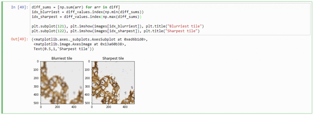
Success! We now have a way to identify the sharpest image in a z-stack, using only free and open source software.

You can download the Jupyter notebook with the code so far here.

Sharpness heatmap

For any z-stacked slide, we can now write a loop that goes over all tiles in the slide. At each location, we retrieve all the z-stacked tiles:

def get_z_stack(path, x, y):
    z_stack = []
    for i in range(0, num_z_stacks):
        # print("getting tile from", path, " at ", x, y, " (zoomlevel", sel_zl, ") / z-stack level ", i)
        z_stack.append(core.get_tile(path, x, y, zoomlevel=sel_zl, zstack=i))
    return z_stack

Now we can calculate at each location independently the sharpest tile.

def determine_sharpest_tile_idx(tiles):
    blur = []
    diff = []

    for idx in range(0, len(tiles)):
        blur.append(cv2.blur(np.array(tiles[idx]),(5,5)))
        diff.append(np.abs(blur[idx] - tiles[idx]))
        diff_sums = [np.sum(arr) for arr in diff]

    return diff_sums.index(np.max(diff_sums))

And we can invoke these method repeatedly for each location in the slide:

zoomlevels = core.get_zoomlevels_dict(slide)
sel_zl = int(round(len(zoomlevels) / 2)) + 2     # arbitrary selection
max_x, max_y = zoomlevels[sel_zl][0], zoomlevels[sel_zl][1]

sharpness_map = []
for x in range(0, max_x):
    print (".", end="")
    for y in range(0, max_y):
        sharpness_map.append(determine_sharpest_tile_idx(get_z_stack(slide, x, y)))

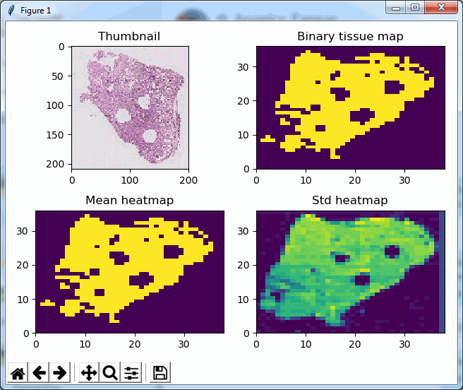
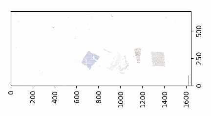
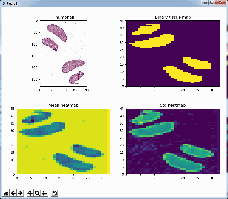
Say that the thumbnail of our image look as follows:

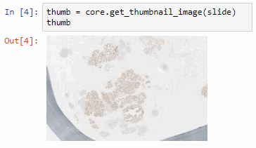
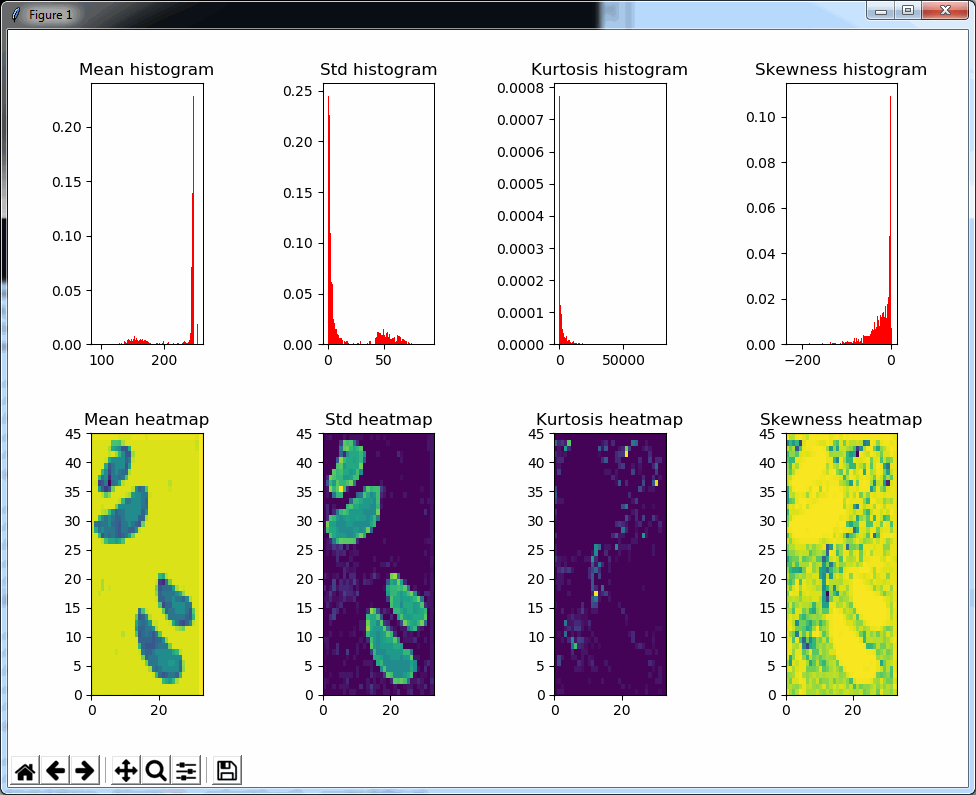
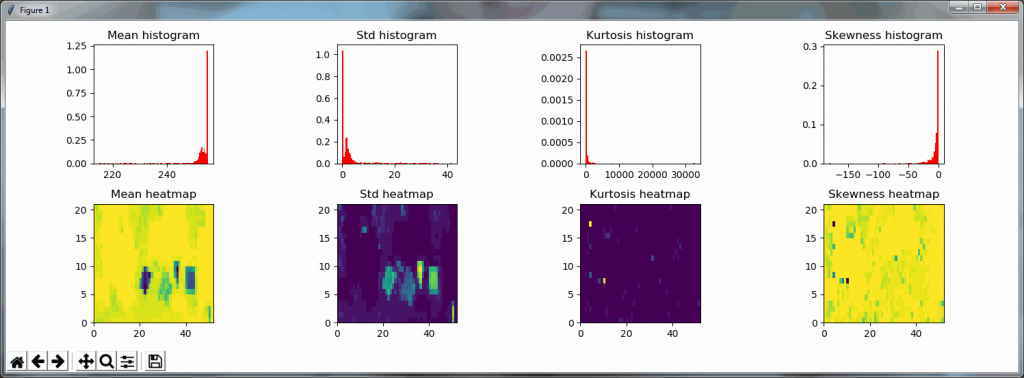
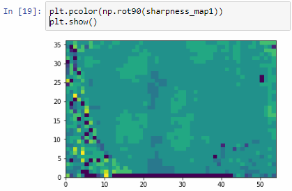
We can then print the selected optimal layers at each position as a heatmap with matplotlib.

The resulting image illustrates the fact that indeed throughout the slide, different clusters of cells are sharper in one plane or another.

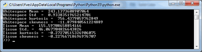
The output for one of our slides looks like this:

Constructing a new single-plane image

Instead of returning the index of the sharpest tile in a stack of tiles, we can return the sharpest tiles itself. For this, we only need to make a small modification in our earlier determine_sharpest_tile_idx function.

def determine_sharpest_tile(tiles):
    blur = []
    diff = []

    for idx in range(0, len(tiles)):
        blur.append(cv2.blur(np.array(tiles[idx]),(5,5)))
        diff.append(np.abs(blur[idx] - tiles[idx]))
        diff_sums = [np.sum(arr) for arr in diff]

    return tiles[diff_sums.index(np.max(diff_sums))]

We can subsequently paste all of the sharpest tiles into a new PIL image object that is made up of the dimensions of the selected zoomlevel from which the tiles are selected:

def get_focused_slide(slide, zoomlevel):
    x_count, y_count, n = core.get_number_of_tiles(slide, zoomlevel)
    x_tile_size, y_tile_size = core.get_tile_size()
    focused_tiles = []
 
    image = Image.new('RGB', (x_count * x_tile_size, y_count * y_tile_size))
 
    coords = list(map(lambda x: (x[0], x[1], zoomlevel), itertools.product(range(y_count), range(x_count))))

    for x in range(0, max_x):
        print (".", end="")
        for y in range(0, max_y):
            focused_tiles.append(determine_sharpest_tile_idx(get_z_stack(slide, x, y)))

    i=0
    for y in range(y_count):
        for x in range(x_count):
            tile = focused_tiles[i]
            i+=1
            image.paste(tile, (x*x_tile_size, y*y_tile_size))

    return image

If you’ve run the code so far, you’ve already found out (the hard way) that it can actually take quite some time to loop over all tiles in the slide this way.

Therefore, let’s introduce some parallellization logic here as well:

def get_focused_tile(c):
    return determine_sharpest_tile(get_z_stack(slide, c[1], c[0], c[2]))

def get_focused_slide(slide, zoomlevel):
    x_count, y_count, n = core.get_number_of_tiles(slide, zoomlevel)
    x_tile_size, y_tile_size = core.get_tile_size()
    focused_tiles = []
 
    image = Image.new('RGB', (x_count * x_tile_size, y_count * y_tile_size))
 
    coords = list(map(lambda x: (x[0], x[1], zoomlevel), itertools.product(range(y_count), range(x_count))))

    tiles = Parallel(n_jobs=-1, verbose=2, backend="threading")(
        map(delayed(get_focused_tile), tqdm(coords)))
 
    i=0
    for y in range(y_count):
        for x in range(x_count):
            tile = tiles[i]
            i+=1
            image.paste(tile, (x*x_tile_size, y*y_tile_size))

    return image

Once you have the new image, saving the image to TIFF output is trivial:

image = get_focused_slide(slide, 6)    # do this at zoomlevel 6, can take a while...
image.save('focused_image.tiff')

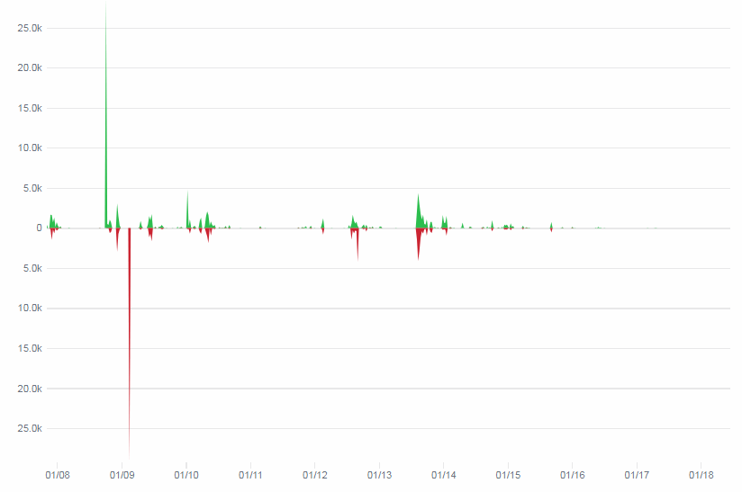
Which in practice can end up looking like this (including parallellization progression bars):

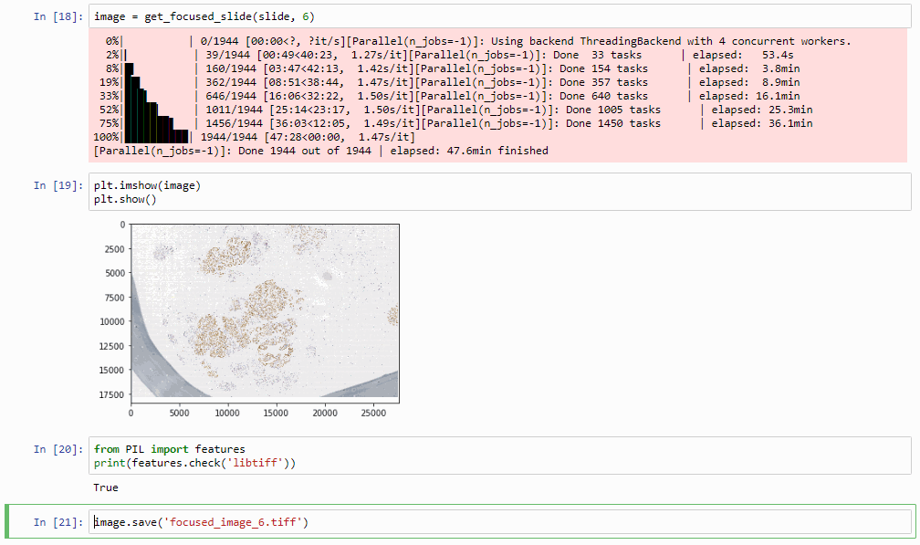
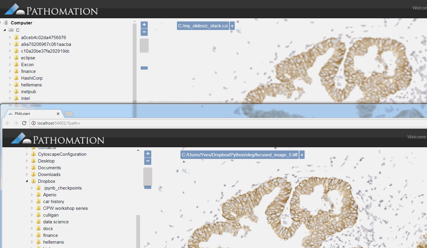
The resulting image can now be opened in turn (in PMA.start, of course) to navigate without the need to continuously having to scan for the sharpest plane.

Here’s comparison of a random zoomlevel in the original image with the same region of interest in the new optimized image:

The sourcecode for this procedure so far can be downloaded as another Jupyter notebook (thanks Oleg Kulaev for helping with the finer details of parallellization and image orientation handling in matplotlib).

Cool huh? Well, sort of, kinda… read on.

Libvips to save our TIFFs

There’s an implicit problem with the TIFFs that we generate: they’re big! Most importantly… they’re flat.

There’s some irony to this. We spent all this effort flattening the z-stacked CZI file for a flat TIFF, which is infinitely slower to navigate than the original CZI!

So saving as a pyramidal TIFF instead of a flat tiff would definitely help our case here.

The quickest way to do this is through libvips, with pyvips bindings installed (make sure that you install libvips before getting pyvips with pip; also, if you’re on Windows, make sure that the libvips’ \bin folder is included in your SYSTEM path variable).

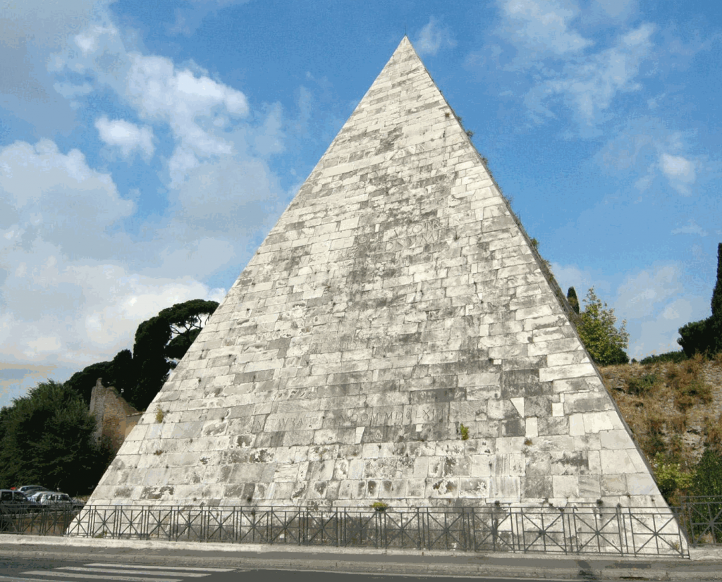
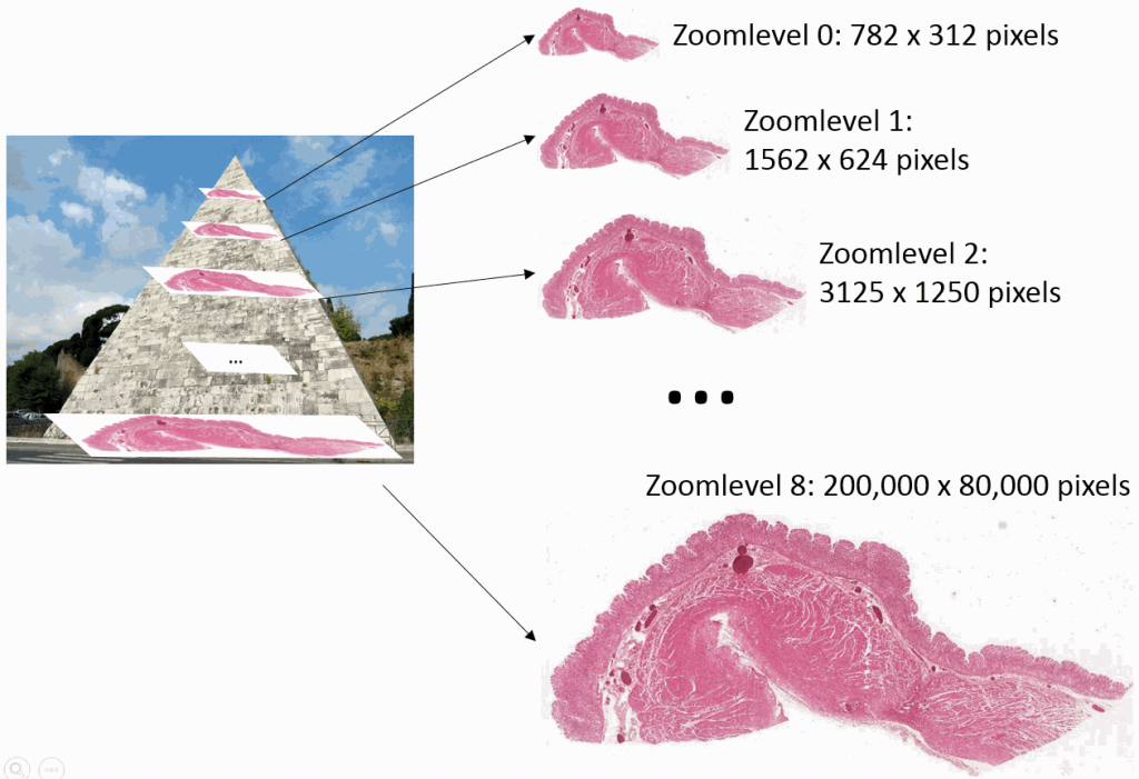
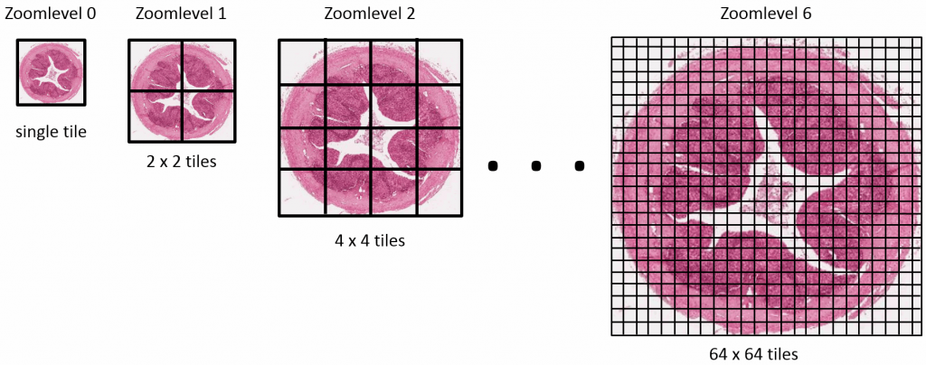
Our final step therefore is getting our “flat” PIL image object to a pyramidal tiff (if you need to freshen up about why the pyramid exists in these files, see our section on Whole Slide Images and pyramid stacks in https://realdata.pathomation.com/digital-microscopy-imaging-data-with-python/)

import pyvips

dtype_to_format = {
 'uint8': 'uchar',
 'int8': 'char',
 'uint16': 'ushort',
 'int16': 'short',
 'uint32': 'uint',
 'int32': 'int',
 'float32': 'float',
 'float64': 'double',
 'complex64': 'complex',
 'complex128': 'dpcomplex',
}

img_3d_array = np.asarray(image)
height, width, bands = img_3d_array.shape
linear = img_3d_array.reshape(width * height * bands)
pyvips_image = pyvips.Image.new_from_memory(linear, width, height, bands, dtype_to_format[str(img_3d_array.dtype)])

tile_width, tile_height = core.get_tile_size()
pyvips_image.write_to_file('pyramidal_image.tiff', tile=True, tile_width=tile_width, tile_height=tile_height, pyramid=True)

This final procedure is available as yet another separate Jupyter notebook. Once again much gratitude goes to Oleg Kulaev for figuring out the libvips interactions.

Curious about how to identify blurry tiles in single plane brightfield images? We have a post about that, too.

Optimization

The procedure as described can still take quite a while to process. The time needed is highly dependent on the selected zoomlevel. Deeper zoomlevels give you better accuracy, but at the expense of having to process more pixels.

We wrote this post mostly to explain the principle of how blur detection and z-stack optimization can work. By no means do we claim that is production-ready code. If you need professional, scalable blur-detection methods, check out e.g. David Ameisen‘s start-up company ImginIT (just don’t expect his process to be as clearly explained as we just did).

Here are a couple of ideas for optimization:

  • Do we really need to consider all pixels in a tile? Can we get by with selecting perhaps every other 2nd, 4th, 8th… pixel perhaps?
  • Do we need to run the blur detection on tiles from zoomlevel x in order to determine the right layer to select from? Perhaps we can get by with zoomlevel x – 1, x – 2…
  • Do we need to process tiles in their entirety? Perhaps we can select tiles from a coarser zoomlevel, artificially break up an individual tiles in smaller tiles, and use those as a reference.
  • Last but not least, do we even need all contingent tiles? This is easiest to illustrate in a 1-dimensional world: if the optimal layer to select from for tile 1 and tile 3 are the same, is there still any point to examine tile 2 as well? It’s easy now to conceive a recursive algorithm that starts with a (possibly even random) selection of tiles that only analyzes intermediate tiles as the need arises.

In a next post we’ll be discussing how you can use PMA.start to generate DICOM-compliant image objects.

Integrity for all

Transferring whole slide images

The following is a cartoon from XKCD dating from a few years back. If you’ve ever been involved in the transfer of whole slide images, this will be very recognizable.

With whole slide imaging data, the above actually is more complicated. The step that is being skipped in the cartoon is the file integrity check. And with whole slide images, as a single virtual slide can consist of multiple files, it can become really complex really fast.

If you’re a professional user of PMA.core, you no doubt have already appreciated the convenience of the “integrity check” tool: it allows you to select a set of slides, and check if they actually really whole slide imaging data.

Can your image management solution do this? 🙂

But we admit, buying PMA.core just to verify virtual slide integrity is probably overkill.

DIY slide integrity

It turns out, PMA.start is just a well capable to verify virtual slide integrity. But first some background about why you would even want to do this.

The fundamental reason why you want to route all of your slide manipulation operations through PMA.start or its bigger brother PMA.core is that the software knows and understands what a slide is. When you copy a number a multi-file slides from one device to another and you refer to our software components in your code for verification purposes, you cannot make any mistakes in terms of accidentally copying only parts of files the slides. If a mistake does crop up in your report, you can simultaneously check whether something was perhaps wrong with the original slides and files. Digital pathology is hard enough as it is; at least do it on a unit of data (the “slide” rather than the “file”) that makes sense!

As much of slide transfers occur “ad hoc” (on a “need to transfer” basis sort of speak), we wrote an integrity check procedure ourselves as an Anaconda Jupyter notebook.

In order to get PMA.python to work with Anaconda, you’ll first have to get it through PyPI. Start an anadonda prompt and type in “pip install pma_python”.

Great, now you’re ready to import our nifty library in your Jupyter notebooks.

Here’s a good way to start all of your notebooks:

The first block confirms the availability of the library; the second block confirms that PMA.start is running on your system.

This is where Jupyter really shines: you can subdivide your Python (or R) code in separate discrete parts and execute them in an order you want. It becomes really convenient to tweak your scripts and even faster to debug them.

Our strategy for doing an integrity check on a folder an its subfolders is straightforward: loop over all the slides in the folder and see whether we can request the slide information from each one:

def loop_over_directories(dir):
    slides = {}
    for subdir in core.get_directories(dir):
        slides.update(loop_over_directories(subdir))
        for slide in core.get_slides(dir):
            slides[slide] = core.get_slide_info(slide)
    return slides

The result of this function is a dictionary that as keys has paths to all the slides, and as values has information objects (or None in case the slide turned out to be corrupt).

We can now invoke the function on an external hard disk’s folder after copying to see if it goes ok. By means of a sanity check, we’ll also output some parameters on the first slide encountered, as well as the number of items in the dictionary:

slides = loop_over_directories("LaCie (F:)/Pathomation")
topslide = slides[list(slides.keys())[0]]
print(topslide["Filename"], topslide["Width"], topslide["Height"])
len(slides)

The output in Jupiter looks like this:

Our next step is to convert part of the dictionary data to a pandas DataFrame, which in turn it written out as an Excel file. The Excel file is subsequently stored on the external hard disk to provide a check-list for the client and confirm data integrity on their end upon receipt.

df = pd.DataFrame(columns=["SlideName", "PixelWidth", "PixelHeight", "ppmX", "ppmY", "SizeOnDisk"])
df.set_index(["SlideName"])
for slide in slides:
    info = slides[slide]
    if info == None:
        print("Unable to get slide information for", slide)
    else:
        df = df.append({"SlideName": slide,
            "PixelWidth": info["Width"],
            "PixelHeight": info["Height"],
            "ppmX": info["MicrometresPerPixelX"],
            "ppmY": info["MicrometresPerPixelY"],
            "SizeOnDisk": info["PhysicalSize"]}, ignore_index=True)
print (df.shape[0], " out of ", len(slides), " check out OK")

Great, but what if things don’t work out they’re supposed to?

As it turns out, we had been copying a collection of slides (about 60GB in total) overnight from an FTP site. Chances are that in the time that takes, something will go wrong. This turned out have happened in our case, as well, and the output flagged correctly that there was a mistake.


The flagged item was minor actually; one of the files had indeed failed to copy and had resulted in a file size with 0 bytes. We downloaded the file anew, and now everything checked out.

Did we need PMA.start to find out that a file was the wrong size? No, we could have used a range of other tools. But the point is that many things can go wrong with whole slide image transfer. The final goal is to check slide integrity, and once a problem is detected, other tools can be used to dig further and resolve them.

There are other potential problems, too: you may be sending someone slides who’s unable to read them. By including a test report from your end with the data, you’re telling them that the files are indeed all right, and that other problems may be at play (perhaps they’re not using the right viewer or import module for the file format that you sent them).

Troubleshooting and debugging is all about eliminating possibilities. We like to think PMA.start (and it’s bigger brother PMA.core) can help you get there faster than anything else on the market today.

You can download the Jupyter notebook discussed in this post. Just modify the folder_to_check variable in the third codeblock to point to the location that you want to validate.


The best kind of criticism

Nothing like honest feedback. I was so happy we finally got something cooking in Pyhon, that I sent it out to couple of people, asking (hoping) for immediate feedback. I failed to provide the full context of PMA.python though. Therefore, here’s one response that I got back:

So there’s obviously a couple of assumptions (leading to misconceptions) about PMA.python that are really easy to make, specifically:

  1. It’s a universal library for whole slide imaging; moreover it’s a self-contained library that doesn’t depend on anything else besides Python itself
  2. PMA.start is a dependency, which is hard to install and set up.
  3. The most important PMA.python dependency, PMA.start, runs on Windows as well as Linux (or Mac)

Lack of information leads to assumptions. Assumptions lead to misconceptions. Misconceptions lead to disappointment. Disappointment leads to anger. Anger leads to hate. Hate leads to suffering.

Aaargh, we single-handedly just tipped the balance of power in the Universe!

But on more serious note:

I hope we successfully prevented people from bumping into 1) by providing additional verbiage in our package description on PyPI:

As for 2) we don’t think this is the case: Downloading a .exe-file and running it is about as easy as we can make it for you. Due to the nature of the software however, the user that installs the software will need administrative access to his or her own computer.

Finally, there 3). We know and we acknowledge the existence of the Linux-community. Unfortunately, porting PMA.start to Linux is not a trivial thing to do. And so, for now, we don’t. We don’t have the resources for that, and we’d rather offer stable software for a single OS, than an average and mediocre  product that nevertheless runs on both. If you’re tied to Linux and require WSI processing with Python, you’ll have to stick with OpenSlide for now (which also requires a separate library to connect to; there simply isn’t a native WSI library for Python).

By the way: the argument actually only partially applies. We offer a commercial version of PMA.core that is not limited to just listening to incoming requests on localhost. PMA.python then can be installed on a Linux datacenter and be used to communicate with the PMA.core instance that hosts the digital slide / tile data. In fact, this is exactly the approach that is being used at CellCarta, Pathomation‘s parent company.

In closing

That being said, we really appreciated the honesty of the poster. The point is: while it’s great to receive positive praise (PMA.start now has about 150 users per month; these can’t all be wrong), it’s the negative criticism that helps you become better and prevents you from becoming complacent.

Update on testing

A performance conundrum

In a previous blog post, we showed how our own software compares to the legacy OpenSlide library. We explained our testing strategy, and did a statistical analysis of the file formats. We analyzed the obtained data for two out of five common WSI file formats.

We subsequently ran the tests for three more formats, but ended up with somewhat of a conundrum. Below are the box and whisker plots for the Leica SCN file format, as well as the 3DHistech MRXS file format. The chart suggests OpenSlide is far superior.

The differences are clear; but at the time so outspoken, that it was unlikely just due to the implementation, especially in light of our results. Case in point: the SCN file format differs little from the SVS format (they’re move adapted and renamed variants of the generic TIFF format).

So we started looking at a higher level of the SCN file that we were using for our analysis. Showing the slide’s meta-data in PMA.core 1, PMA.core 1 + OpenSlide, and PMA.core 2. As PMA.core 1 and PMA.core 2 show similar performance, we only include PMA.core 2 (on the right) in the screenshot below.

What happens is that PMA.core 2 only identifies the tissue on the glass, while OpenSlide not only identifies the tissue, but also builds a virtual whitespace area around the slide. This representation of the slide in OpenSlide is therefore much larger than the representation of slide in PMA.core (even though we’re talking about the same slide). The pixel space is with OpenSlide is almost 6 times bigger (5.76 times to be exact); but all of that extra space are just empty tiles.

Now when we’re doing random sampling of tiles, we select from the entire pixel space. So, by chance, when selecting random tiles from the OpenSlide rendering engine, we’re much more likely to end up with an empty tile, than with PMA.core. Tiles get send back to the client in JPEG files, and blank tiles can be compressed and reduced in size much more than actual tissue tiles. We looked at the histogram and cumulative frequency distribution of pixel values in our latest post.

The same logic applies to the MRXS format: A side by side comparison also reveals that the pixel space in the OpenSlide build is much larger than in PMA.core.

The increased chance of ending up with a blank tile instead of real tissue doesn’t just explain the difference in mean retrieval times, it also explains the difference in variance that can be seen in the box and whisker plots.

Is_tissue() to the rescue

But wait, we just wrote that is_tissue() function earlier, that let’s us detect whether an obtained tile is blank or has tissue in it, right? Let’s use that one to see if a tile is whitespace or tissue. If it is tissue, we count the result in our statistic, it it’s not, we leave it out, and continue until we do hit a tissue tile that is worthy of inclusion.

To recap, here’s the code to our is_tissue() function (which we can’t condone for general use, but it’s good enough to get the job done here):

def is_tissue(tile):
    pixels = np.array(tile).flatten()        # np refers to numpy
    mean_threahold = np.mean(pixels) < 192   # 75th percentile
    std_threshold = np.std(pixels) < 75
    return mean_threahold == True and std_threshold == True

And our code for tile retrieval becomes like this:

def get_tiles(server, user, pwd, slide, num_trials = 100):
    session_id = pma.connect(server, user, pwd)
    print ("Obtained Session ID: ", session_id)
    info = pma.get_slide_info(slide, session_id)
    timepoints = []
    zl = pma.get_max_zoomlevel(slide, session_id)
    print("\t+getting random tiles from zoomlevel ", zl)
    (xtiles, ytiles, _) = pma.get_zoomlevels_dict(slide, session_id)[zl]
    total_tiles_requested = 0
    while len(timepoints) <= num_trials:
        xtile = randint(0, xtiles)
        ytile = randint(0, ytiles)
        print ("\t+getting tile ", len(timepoints), ":", xtile, ytile)
        s_time = datetime.datetime.now()    # start_time
        tile = pma.get_tile(slide, xtile + x, ytile + y, zl, session_id)
        total_tiles_requested = total_tiles_requested + 1
        if is_tissue(tile):
            timepoints.append((datetime.datetime.now() - s_time).total_seconds())
    pma.disconnect(session_id)
    print(total_tiles_requested, “ number of total tiles requested”)
    return timepoints

Note that at the end of our test function, we print out how many tiles we actually had to retrieve from each slide, in order to reach a sampling size that matches the trial_size parameter.

Running this on the MRXS sample both in our OpenSlide build and PMA.core 2 confirms our hypothesis about the increase in pixel space (and a bias for empty tiles). In our OpenSlide build, we have to weed through 4200 tiles to get a sample of 200 tissue tiles; in PMA.core 2 we “only” require 978 iterations.

Plotting the results as a box and whisker chart, we now get:

We turn to statistics once again to support our hypothesis:

We can do the same for SCN now. First, let’s see if we can indeed use the Is_Tissue() function to on the slide as a filter:

This looks good, and we run the same script as earlier. We notice the same discrepancy of overrepresented blank tiles in the SCN file when using OpenSlide. In our OpenSlide build, we have to retrieve 3111 tiles. Using our own implementation, only 563 tiles are needed.

When we do a box and whisker plot, we confirm the superior performance of PMA.core compared to OpenSlide:

The statistics further confirm the observations of the box and whisker plot (p-value of 0.004 when examining the difference in means):

What does it all mean?

We generated all of the above and previous statistics and test suites to confirm that our technology is indeed faster than the legacy OpenSlide library. We did this on three different versions of PMA.core: version 1.2, a custom build of version 1.2 using OpenSlide where possible, and PMA.core 2.0 (currently under development). We can summarize our findings like this:

Note that we had to modify our testing strategy slightly for MRXS and SCN. The table doesn’t really suggest that it takes twice as long to read an SCN file compare to an SVSlide file. The discrepancies between the different file formats is the result of selecting either only tissue slides (MRXS, SCN), or a random mixture of both tissue and blank tiles.

When requesting tiles in a sequential manner (we’ll come back to parallel data retrieval in the future), the big takeaway number is that PMA.core is on average 11% faster than OpenSlide.


Dude, where’s my tissue?

Whitespace and tissue

Let’s say that you have a great algorithms to distinguish between PDL1- and a CD8-stained cells.

Your first challenge to run this on real data, is to find the actual tiles that contain tissue, rather than just whitespace. This is because your algorithm might be computationally expensive, and therefore you want to run it only on parts of the slide where it makes sense to do the analysis. In order words: you want to eliminate the whitespace.

At our PMA.start website, you can find OpenCV code that automatically outlines an area of tissue on a slide, but in this post we want to tackle things at a somewhat more fundamental level.

Let’s see if we can figure out a mechanism ourselves to distinguish tissue from whitespace.

First, we need to do some empirical exploration. So let’s start by downloading a reference slide from OpenSlide and request its thumbnail through PMA.start:

from pma_python import core
slide = "C:/my_slides/CMU-1.svs"
core.get_thumbnail_image(slide).show()

As we can see, there’s plenty of whitespace to go around. Let’s get a whitespace tile at position (0,0), and a tissue tile at position (max_x / 4, max_y / 2). Intuitively you may want to go for (max_x/2, max_y/2), but that wouldn’t get us anywhere here. So pulling up the thumbnail first is important for this exercise, should you do this on a slide of your own (and your coordinates may vary from ours).

Displaying these tiles two example tiles side by side goes like this:

from pma_python import core
slide = "C:/my_slides/CMU-1.svs"
max_zl = core.get_max_zoomlevel(slide)
dims = core.get_zoomlevels_dict(slide)[max_zl]

tile_0_0 = core.get_tile(slide, x=0, y=0, zoomlevel=max_zl)
tile_0_0.show()

tile_x_y = core.get_tile(slide, x=int(dims[0] / 4), y=int(dims[1] / 2), zoomlevel=max_zl)
tile_x_y.show()

And looks like this:

Now that we have the two distinctive tiles, let’s convert both to grayscale and add a histogram to our script for each:

from pma_python import core
import matplotlib.pyplot as plt
import numpy as np

slide = "C:/my_slides/CMU-1.svs"
max_zl = core.get_max_zoomlevel(slide)
dims = core.get_zoomlevels_dict(slide)[max_zl]

# obtain whitespace tile
tile_0_0 = core.get_tile(slide, x=0, y=0, zoomlevel=max_zl)
# Flatten the whitespace into 1 dimension: pixels
pixels_0_0 = np.array(tile_0_0).flatten()

# obtain tissue tile
tile_x_y = core.get_tile(slide, x=int(dims[0] / 4), y=int(dims[1] / 2), zoomlevel=max_zl)
# Flatten the tissue into 1 dimension: pixels
pixels_x_y = np.array(tile_x_y).flatten()

# Display whitespace image
plt.subplot(2,2,1)
plt.title('Whitespace image')
plt.axis('off')
plt.imshow(tile_0_0, cmap="gray")

# Display a histogram of whitespace pixels
plt.subplot(2,2,2)
plt.xlim((0,255))
plt.title('Whitespace histogram')
plt.hist(pixels_0_0, bins=64, range=(0,256), color="red", alpha=0.4, normed=True)

# Display tissue image
plt.subplot(2,2,3)
plt.title('Tissue image')
plt.axis('off')
plt.imshow(tile_x_y, cmap="gray")

# Display a histogram of whitespace pixels
plt.subplot(2,2,4)
plt.xlim((0,255))
plt.title('Tissue histogram')
plt.hist(pixels_x_y, bins=64, range=(0,256), color="red", alpha=0.4, normed=True)

# Display the plot
plt.tight_layout()
plt.show()

As you can see, we make use of PyPlot subplots here. The output looks as follows, and shows how distinctive the histogram for whitespace is compared to actual tissue areas.

We can add a cumulative distribution function to further illustrate the difference:

# Display whitespace image
plt.subplot(2,3,1)
plt.title('Whitespace image')
plt.axis('off')
plt.imshow(tile_0_0, cmap="gray")

# Display a histogram of whitespace pixels
plt.subplot(2,3,2)
plt.xlim((0,255))
plt.title('Whitespace histogram')
plt.hist(pixels_0_0, bins=64, range=(0,256), color="red", alpha=0.4, normed=True)

# Display a cumulative histogram of the whitespace
plt.subplot(2,3,3)
plt.hist(pixels_0_0, bins=64, range=(0,256), normed=True, cumulative=True, color='blue')
plt.xlim((0,255))
plt.grid('off')
plt.title('Whitespace CDF')

# Display tissue image
plt.subplot(2,3,4)
plt.title('Tissue image')
plt.axis('off')
plt.imshow(tile_x_y, cmap="gray")

# Display a histogram of whitespace pixels
plt.subplot(2,3,5)
plt.xlim((0,255))
plt.title('Tissue histogram')
plt.hist(pixels_x_y, bins=64, range=(0,256), color="red", alpha=0.4, normed=True)

# Display a cumulative histogram of the tissue
plt.subplot(2,3,6)
plt.hist(pixels_x_y, bins=64, range=(0,256), normed=True, cumulative=True, color='blue')
plt.xlim((0,255))
plt.grid('off')
plt.title('Tissue CDF')

Note that we’re now using a 2 x 3 grid to display the histogram and the cumulative distribution function (CDF) next to each other, which ends up looking like this:

Back to basic (statistics)

We could now write a complicated method that manually scans through the pixel-arrays and assesses how many bins there are, how they are distributed etc. However, it is worth noting that the histogram-buckets that are NOT showing any values in the histogram, are not pixels-values of 0; the histogram shows a frequency, therefore, empty spaces in the histogram simply means that NO pixels are available at a given intensity.

So after we visualized the pixel distribution through MatPlotLib’s PyPlot, it’s worth looking as some basic statistics for the flattened pixels arrays. Numpy’s basic .std() and .mean() functions are good enough to do the job for now. The script becomes:

from pma_python import core
import matplotlib.pyplot as plt
import numpy as np
import scipy.stats

slide = "C:/my_slides/CMU-1.svs"
max_zl = core.get_max_zoomlevel(slide)
dims = core.get_zoomlevels_dict(slide)[max_zl]

# obtain whitespace tile
tile_0_0 = core.get_tile(slide, x=0, y=0, zoomlevel=max_zl)
# Flatten the whitespace into 1 dimension: pixels
pixels_0_0 = np.array(tile_0_0).flatten()
# print whitespace statistics
print("Whitespace Mean = ", np.mean(pixels_0_0))
print("Whitespace Std  = ", np.std(pixels_0_0))
print("Whitespace kurtosis = ", scipy.stats.kurtosis(pixels_0_0))
print("Whitespace skewness = ", scipy.stats.skew(pixels_0_0))

# obtain tissue tile
tile_x_y = core.get_tile(slide, x=int(dims[0] / 4), y=int(dims[1] / 2), zoomlevel=max_zl)
# Flatten the tissue into 1 dimension: pixels
pixels_x_y = np.array(tile_x_y).flatten()
# print tissue statistics
print("Tissue Mean = ", np.mean(pixels_x_y))
print("Tissue Std. = ", np.std(pixels_x_y))
print("Tissue kurtosis = ", scipy.stats.kurtosis(pixels_x_y))
print("Tissue skewness = ", scipy.stats.skew(pixels_x_y))

The output (for the same tiles as we visualized using PyPlot earlier is as follows:

The numbers suggest that the mean-(grayscale-)value of a Whitespace tile is a lot higher than that of a tissue tile. More importantly: the standard deviation (variance squared) could be an even more important indicator. Naturally we would expect the standard deviation of (homogenous) whitespace to be much less than that of tissue pictures containing a range of different features.

Kurtosis and skewness are harder to interpret and place, but let’s keep them in there for our further investigation below.

Another histogram

We started this post by analyzing an individual tile’s grayscale histogram. We now summarized that same histogram in a limited number of statistical measurements. In order to determine whether those statistical calculations are an accurate substitute for a visual inspection, we compute those parameters for each tile at a zoomlevel, and then plot those data as a heatmap.

The script for this is as follows. Depending on your fast your machine is, you can play w/ the zoomlevel parameter at the top of the script, or set it to the maximum zoomlevel (at which point you’ll be evaluating every pixel in the slide.

from pma_python import core
import matplotlib.pyplot as plt
import numpy as np
import scipy.stats
import sys

slide = "C:/my_slides/CMU-1.svs"
max_zl = 6 # or set to core.get_max_zoomlevel(slide)
dims = core.get_zoomlevels_dict(slide)[max_zl]

means = []
stds = []
kurts = []
skews = []

for x in range(0, dims[0]):
    for y in range(0, dims[1]):
        tile = core.get_tile(slide, x=x, y=y, zoomlevel=max_zl)
        pixels = np.array(tile).flatten()
        means.append(np.mean(pixels))
        stds.append(np.std(pixels))
        kurts.append(scipy.stats.kurtosis(pixels))
        skews.append(scipy.stats.skew(pixels))
    print(".", end="")
    sys.stdout.flush()
print()

means_hm = np.array(means).reshape(dims[0],dims[1])
stds_hm = np.array(stds).reshape(dims[0],dims[1])
kurts_hm = np.array(kurts).reshape(dims[0],dims[1])
skews_hm = np.array(skews).reshape(dims[0],dims[1])

plt.subplot(2,4,1)
plt.title('Mean histogram')
plt.hist(means, bins=100, color="red", normed=True)
plt.subplot(2,4,5)
plt.title('Mean heatmap')
plt.pcolor(means_hm)

plt.subplot(2,4,2)
plt.title('Std histogram')
plt.hist(stds, bins=100, color="red", normed=True)
plt.subplot(2,4,6)
plt.title("Std heatmap")
plt.pcolor(stds_hm)

plt.subplot(2,4,3)
plt.title('Kurtosis histogram')
plt.hist(kurts, bins=100, color="red", normed=True)
plt.subplot(2,4,7)
plt.title("Kurtosis heatmap")
plt.pcolor(kurts_hm)

plt.subplot(2,4,4)
plt.title('Skewness histogram')
plt.hist(skews, bins=100, color="red", normed=True)
plt.subplot(2,4,8)
plt.title("Skewness heatmap")
plt.pcolor(skews_hm)

plt.tight_layout()
plt.show()

The result is a 2 row x 4 columns PyPlot grid, shown below for a selected zoomlevel of 6:

The standard deviation as well as the mean grayscale value of a tile seem accurate indicators to determine the position of where tissue can be found on the slide; skewness and kurtosis not so much.

Both the mean histogram and the standard deviation histogram show a bimodal distribution, and we can confirm their behavior by looking at other slides. It even works on slides that are only lightly stained (we will return to these at a later post and see how we can make the detection better in these:

A binary map

We can now write a function that determines whether a tile is (mostly) tissue, based on the mean and standard deviation of the grayscale pixel values, like this:

def is_tissue(tile):
    pixels = np.array(tile).flatten()
    mean_threahold = np.mean(pixels) < 192   # 75th percentile
    std_threshold = np.std(pixels) < 75
    return mean_threahold == True and std_threshold == True

Writing a similar function that determines whether a tile is (mostly) whitespace, is possible, too, of course:

def is_whitespace(tile):
    return not is_tissue(tile)

Similarly, we can even use this function to now construct a black and white map of where the tissue is located on a slide. The default color map of PyPlot on our system nevertheless rendered the map blue and yellow:

In closing

This post started with “Let’s say that you have a great algorithms to distinguish between PDL1- and a CD8-stained cells.”. We didn’t quite solve that challenge yet. But we did show you some important initial steps you’ll have to take to get to that part eventually.

In the next couple of blogs we want to elaborate on the topic of tissue detection some more. We want to discuss different types of input material, as well as see if we can use a machine learning classifier to replace the deterministic mapping procedure developed here.

But first, we’ll get back to testing, and we’ll tell you why it was important to have the is_tissue() function from the last paragraph developed first.

To OpenSlide or not to OpenSlide

The legacy

When you say digital pathology or whole slide imaging, sooner or later you end up with OpenSlide. This is essentially a programming library. Back in 2012, a pathologist alerted me to it (there’s some irony to the fact that he found it before me, the bioinformatician). He didn’t know what to do with it, but it looked interesting to him.

OpenSlide is how Pathomation got started. We actually contributed to the project.

We also submitted sample files to add to their public repository (and today, we use this repository frequently ourselves, as do many others, I’m sure).

Our names are mentioned in the Acknowledgements section of the OpenSlide paper.

But today, the project has rather slowed down. This is easy to track through their GitHub activity page:

Kudos to the team; they do still make an effort to fix bugs that crop up, today’s but activities seem limited to maintenance. Of course there’s a possibility that nobody gets the code through GitHub anymore, but rather through one of the affiliate projects that they are embedded into.

Consider this though: OpenSlide Discussions about supporting support for (immuno)fluorescence and z-stacking date back to 2012  , but never resulted in anything. Similarly, there are probably about a dozen file formats out there that they don’t support (or flavors that they don’t support, like Sakura’s SVSlide format, which was recently redesigned). We made a table of the formats that we support, and they don’t, at http://free.pathomation.com/pma_start_omero_openslide/

Free at last

Our own software, we’re proud to say, is OpenSlide-free. PMA.start no longer ships with the OpenSlide binaries. The evolution our software has gone through then is as follows (the table doesn’t list all the formats we support; for a full list see http://free.pathomation.com/formats):

At one time, we realized there was really only one file format left that we still ran through OpenSlide, and with the move to cloud storage (more on that in a later post), we decided we might as well make one final effort to re-implement a parser for 3DHistech MRXS slides ourselves.

Profiling

Of course all of this moving away from OpenSlide is useless if we don’t measure up in terms of performance.

So here’s what we did: we downloaded a number of reference slides from the OpenSlide website. Then, we took our latest GAMP5 validated version of our PMA.core 1.2 software, and rerouted it’s slide parsing routines to OpenSlide. This result in a PMA.core 1.2 build that instead of just 2 (Sakura SVSlide and 3DHistech MRXS), now reads 5 different WSI file formats through OpenSlide:  Sakura SVSlide, 3DHistech MRXS, Leica SCN, Aperio SVS, and Hamamatsu NDPI.

Our test methodology consist of the following steps:

For each slide:
    Determine the deepest zoomlevel
    From this zoomlevel select 200 random tiles
    Retrieve each tile sequentially
    Keep track of how long it takes to retrieve each tiles

We run this scenario of 3 instances of PMA.core:

  •                 PMA.core 1.2 without OpenSlide (except for SVSlide and MRXS)
  •                 PMA.core 1.2 custom-build with OpenSlide (for all 5 file formats)
  •                 PMA.core 2 beta without OpenSlide

The random tiles selected from the respective slides are different each time. The tiles extracted from slide.ext on PMA.core instance 1 are different from the ones retrieved through PMA.core instance 2.

Results

As simple as the above script sounds, we discovered some oddities while running them for each file format.

Let’s start w/ the two easiest to explain ones: SVS and SVSlide.

A histogram of the recorded times for SVSlide yields the following chart:

We can see visually that PMA.core 1.2 without OpenSlide is a little faster than the PMA.core 1.2 custom-build with OpenSlide, and that we were able to improve this performance yet again in PMA.core 2.

The p-value confirm this. First we do an F-test to determine what T-test we need (p-values of 1.66303E-78 and 2.03369E-05 suggests inequal variances),

Next, we find a p-value of 0.859 (n=200) for the difference in mean tile retrieval time between PMA.core 1.2 with and without OpenSlide, and a p-value of 2.363E-06 for the difference in means between PMA.core 1.2 with OpenSlide and PMA.core 2 without OpenSlide.

We see this as conclusive evidence that PMA.core 2 (as well as PMA.start, which contains a limited version of the PMA.core 2 code in the form of PMA.core.lite) can render tiles faster than OpenSlide can.

What about SVSlide?

Again, let’s start by looking at the histogram:

This is the same trend as we saw for SVS, so let’s see if we can confirm this with statistics. The F-statistic between PMA.core 1.2 with and without OpenSlide yields a p-value of 3.064E-22; between PMA.core 1.2 without OpenSlide and PMA.core 2 we get a p-value of 3.068E-13.

Subsequent T-tests (assuming unequal variance) between PMA.core 1.2 with and without OpenSlide show a p-value of  8.031E-19; between PMA.core 1.2 with OpenSlide and PMA.core 2 we get a p-value of 4.10521E-17 (one-tailed).

Again, we conclude that both PMA.core 1.2 and PMA.core 2 (as well as PMA.start) are faster to render Sakura SVSlide slides than OpenSlide.

What about the others?

We’re still working on getting data for the other file formats. Stay tuned!