A performance conundrum

In a previous blog post, we showed how our own software compares to the legacy OpenSlide library. We explained our testing strategy, and did a statistical analysis of the file formats. We analyzed the obtained data for two out of five common WSI file formats.

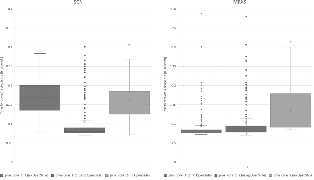
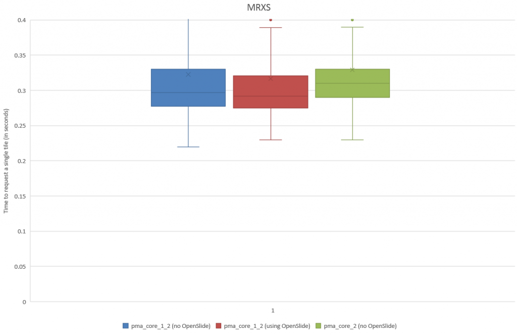
We subsequently ran the tests for three more formats, but ended up with somewhat of a conundrum. Below are the box and whisker plots for the Leica SCN file format, as well as the 3DHistech MRXS file format. The chart suggests OpenSlide is far superior.

The differences are clear; but at the time so outspoken, that it was unlikely just due to the implementation, especially in light of our results. Case in point: the SCN file format differs little from the SVS format (they’re move adapted and renamed variants of the generic TIFF format).

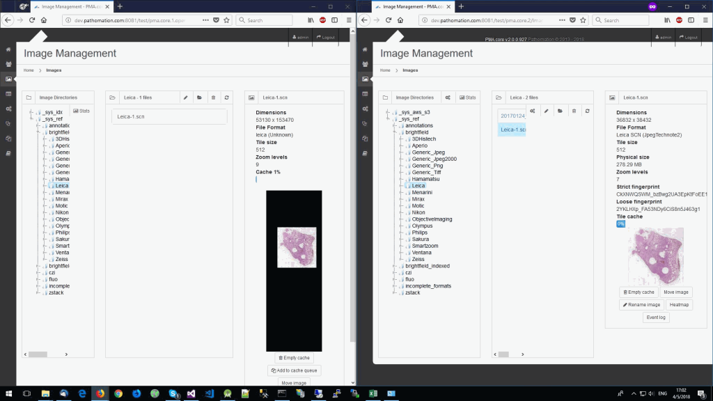
So we started looking at a higher level of the SCN file that we were using for our analysis. Showing the slide’s meta-data in PMA.core 1, PMA.core 1 + OpenSlide, and PMA.core 2. As PMA.core 1 and PMA.core 2 show similar performance, we only include PMA.core 2 (on the right) in the screenshot below.

What happens is that PMA.core 2 only identifies the tissue on the glass, while OpenSlide not only identifies the tissue, but also builds a virtual whitespace area around the slide. This representation of the slide in OpenSlide is therefore much larger than the representation of slide in PMA.core (even though we’re talking about the same slide). The pixel space is with OpenSlide is almost 6 times bigger (5.76 times to be exact); but all of that extra space are just empty tiles.

Now when we’re doing random sampling of tiles, we select from the entire pixel space. So, by chance, when selecting random tiles from the OpenSlide rendering engine, we’re much more likely to end up with an empty tile, than with PMA.core. Tiles get send back to the client in JPEG files, and blank tiles can be compressed and reduced in size much more than actual tissue tiles. We looked at the histogram and cumulative frequency distribution of pixel values in our latest post.

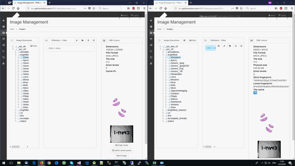
The same logic applies to the MRXS format: A side by side comparison also reveals that the pixel space in the OpenSlide build is much larger than in PMA.core.

The increased chance of ending up with a blank tile instead of real tissue doesn’t just explain the difference in mean retrieval times, it also explains the difference in variance that can be seen in the box and whisker plots.

Is_tissue() to the rescue

But wait, we just wrote that is_tissue() function earlier, that let’s us detect whether an obtained tile is blank or has tissue in it, right? Let’s use that one to see if a tile is whitespace or tissue. If it is tissue, we count the result in our statistic, it it’s not, we leave it out, and continue until we do hit a tissue tile that is worthy of inclusion.

To recap, here’s the code to our is_tissue() function (which we can’t condone for general use, but it’s good enough to get the job done here):

def is_tissue(tile):
    pixels = np.array(tile).flatten()        # np refers to numpy
    mean_threahold = np.mean(pixels) < 192   # 75th percentile
    std_threshold = np.std(pixels) < 75
    return mean_threahold == True and std_threshold == True

And our code for tile retrieval becomes like this:

def get_tiles(server, user, pwd, slide, num_trials = 100):
    session_id = pma.connect(server, user, pwd)
    print ("Obtained Session ID: ", session_id)
    info = pma.get_slide_info(slide, session_id)
    timepoints = []
    zl = pma.get_max_zoomlevel(slide, session_id)
    print("\t+getting random tiles from zoomlevel ", zl)
    (xtiles, ytiles, _) = pma.get_zoomlevels_dict(slide, session_id)[zl]
    total_tiles_requested = 0
    while len(timepoints) <= num_trials:
        xtile = randint(0, xtiles)
        ytile = randint(0, ytiles)
        print ("\t+getting tile ", len(timepoints), ":", xtile, ytile)
        s_time = datetime.datetime.now()    # start_time
        tile = pma.get_tile(slide, xtile + x, ytile + y, zl, session_id)
        total_tiles_requested = total_tiles_requested + 1
        if is_tissue(tile):
            timepoints.append((datetime.datetime.now() - s_time).total_seconds())
    pma.disconnect(session_id)
    print(total_tiles_requested, “ number of total tiles requested”)
    return timepoints

Note that at the end of our test function, we print out how many tiles we actually had to retrieve from each slide, in order to reach a sampling size that matches the trial_size parameter.

Running this on the MRXS sample both in our OpenSlide build and PMA.core 2 confirms our hypothesis about the increase in pixel space (and a bias for empty tiles). In our OpenSlide build, we have to weed through 4200 tiles to get a sample of 200 tissue tiles; in PMA.core 2 we “only” require 978 iterations.

Plotting the results as a box and whisker chart, we now get:

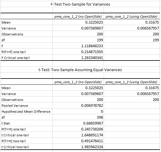
We turn to statistics once again to support our hypothesis:

We can do the same for SCN now. First, let’s see if we can indeed use the Is_Tissue() function to on the slide as a filter:

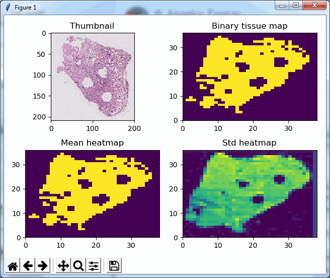
This looks good, and we run the same script as earlier. We notice the same discrepancy of overrepresented blank tiles in the SCN file when using OpenSlide. In our OpenSlide build, we have to retrieve 3111 tiles. Using our own implementation, only 563 tiles are needed.

When we do a box and whisker plot, we confirm the superior performance of PMA.core compared to OpenSlide:

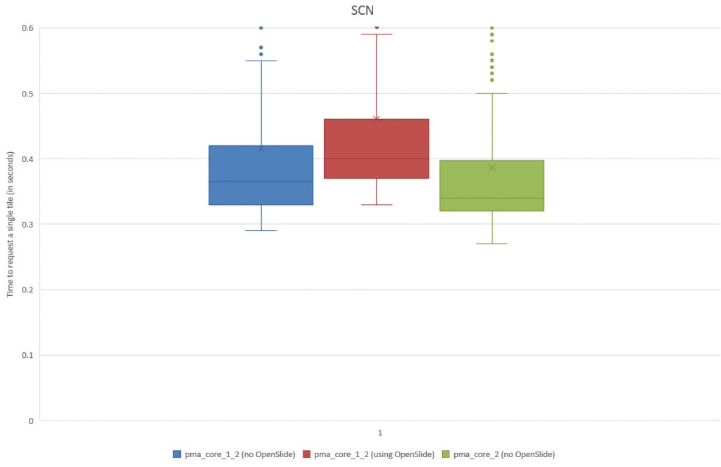
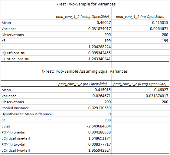
The statistics further confirm the observations of the box and whisker plot (p-value of 0.004 when examining the difference in means):

What does it all mean?

We generated all of the above and previous statistics and test suites to confirm that our technology is indeed faster than the legacy OpenSlide library. We did this on three different versions of PMA.core: version 1.2, a custom build of version 1.2 using OpenSlide where possible, and PMA.core 2.0 (currently under development). We can summarize our findings like this:

Note that we had to modify our testing strategy slightly for MRXS and SCN. The table doesn’t really suggest that it takes twice as long to read an SCN file compare to an SVSlide file. The discrepancies between the different file formats is the result of selecting either only tissue slides (MRXS, SCN), or a random mixture of both tissue and blank tiles.

When requesting tiles in a sequential manner (we’ll come back to parallel data retrieval in the future), the big takeaway number is that PMA.core is on average 11% faster than OpenSlide.