Tile servers and tiles

The Pathomation API and SDKs are built around tiles. PMA.start and PMA.core are essentially tile servers. Conceptually, Whole Slide Imaging servers are not that different from GIS software. Putting it in big data terms, the difference between the two often lies in the Velocity of the data; GIS software has the luxury of being concerned with only one planet Earth, whereas a totally new whole slide image is generated every couple of minutes or so. Say what you will; exo-planets will never be mapped at the speed of tissue.

This impacts how the two categories of software can (afford to) manipulate tiles behind the scenes. Data duplication of Planet Earth’s satellite imagery is acceptable if it speeds up the graphics rendering process. In contrast, this is not the case for whole slide images. Because of the amount of data generated in a short timeframe, storage and time needed to extract all tiles beforehand registered somewhere on a scale from unnecessary, over impractical, up to just downright impossible.

That being said, a tile is valuable. It took time to extract and to render, and it will be gone once you release it, so you better do something useful with it once you have it!

What’s in a tile?

A tile in Pathomation is typically 500 by 500 pixels. That’s actually a LOT of pixels (250,000). Add to that the fact that we’re usually talking about 24-bit data stored in the RGB color space, and you end up with 750,000 bytes needed to store a single tile in-memory. It also means that when we compute an individual tile’s histogram, we need no fewer than 750,000 computations to take place. If you have a grid of 1000 x 2000 tiles… you do the math.

But of course, today’s GPUs solve all this for you, right? We can do billions of computations per second. We have gigabytes of RAM memory available, and it’s all cheap. Why even bother button up the original slide in tiles at all?

Because algorithms and optimization still matter. At our recent CPW2018 workshop, one very clear message was that we cannot solve problems in pathology by brute force. Knowing what happens behind the scenes is still relevant.

In an AI-centric world, deep learning (DL) is at the center of that center. Can we really solve all problems in the world by just adding more layers to our networks?

With real problems, can we even afford to waste C/GPU cycles using brute force “throw enough at the wall; something will stick” approaches? Or did XKCD essentially get it right when they illustrated the goal of technology?

So, this is just a long rant to illustrate our point that we think it’s still worthwhile to think about proper algorithmic design and parallelization. The tile as a basic unit is key to that, and our software can help you get bite-size tiles for your processing pleasure.

Loading images and tiles

If you’ve made it this far, it means you at least partially agree with out tile-centric vision. Cool! Perhaps you’ve even tried a couple of our code snippets in our earlier tutorials already. Even cooler! Perhaps you’ve already experienced how SLOW some of our proposed solutions to problems are. In the latter: stick with us; we totally plan on addressing all of these issues in the coming months through posts examining various aspects of these problems.

Before we get into this however, let’s just explore some of the basic techniques there are in Python to work with partial image content. Here’s how we can load an image from disk:

import matplotlib.pyplot as plt
img_grid = plt.imread("ref_grid.png")
plt.imshow(img_grid)

And here’s how we can load a tile through Pathomation:

from pma_python import core
core.connect()    # connect to PMA.start
img_tile = core.get_tile("C:/my_slides/CMU-1.svs")   # make sure this file exists on your HDD
plt.imshow(img_tile)

The internal Python representations are slightly different:

print(type(img_grid))
print(type(img_tile))

But we can convert PIL image-objects to Numpy arrays just as easily. We can convert an image to a numpy array, and subsequently visualize that one:

import numpy as np
arr_tile = np.array(img_tile)
print(type(arr_tile))
plt.imshow(arr_tile)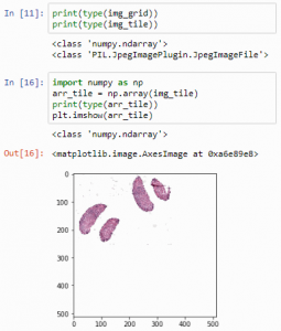

Converting a numpy ndarray back to a PIL Image goes like this:

import numpy as np
type(arr_grid)
pil_grid = Image.fromarray(np.uint8(arr_grid))
type(pil_grid)

Take a note of this! There’s a tremendous amount of operations possible in Python, but some of it is in numpy, other things occur in matplotlib, there’s PIL etc. Chances are that you’ll be converting back and forth between different types quite often.

Subplots

Matplotlib offers a convenient way to combine multiple images into a grid-like organization:

import matplotlib.pyplot as plt
from pma_python import core
core.connect()    # connect to PMA.start

img_tile1 = core.get_tile("C:/my_slides/CMU-1.svs", zoomlevel = 0)
img_tile2 = core.get_tile("C:/my_slides/CMU-1.svs", zoomlevel = 1)
img_tile3 = core.get_tile("C:/my_slides/CMU-1.svs", zoomlevel = 2)

plt.subplot(1,3,1)
plt.imshow(img_tile1)
plt.subplot(1,3,2)
plt.imshow(img_tile2)
plt.subplot(1,3,3)
plt.imshow(img_tile3)

plt.show()

And here’s a one more neat trick:

def plot_slide_as_tiles(slide_ref, zoomlevel):
    dims = core.get_zoomlevels_dict(slide_ref)[zoomlevel]
    max_x = dims[0]
    max_y = dims[1]
    plt.subplots(max_y, max_x, figsize=(15,15))
    for x in range(0,max_x):
        for y in range(0,max_y):
            plt.subplot(max_y, max_x, (x+1) + y * max_x)
            plt.imshow(core.get_tile(slide_ref, zoomlevel = zoomlevel, x = x, y = y))
    plt.plot(figsize=(200,100))
plt.show()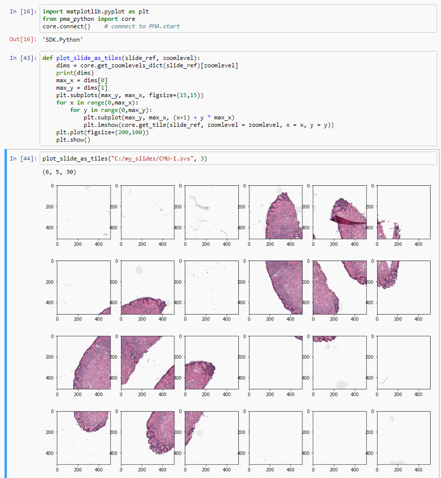

Basic operations

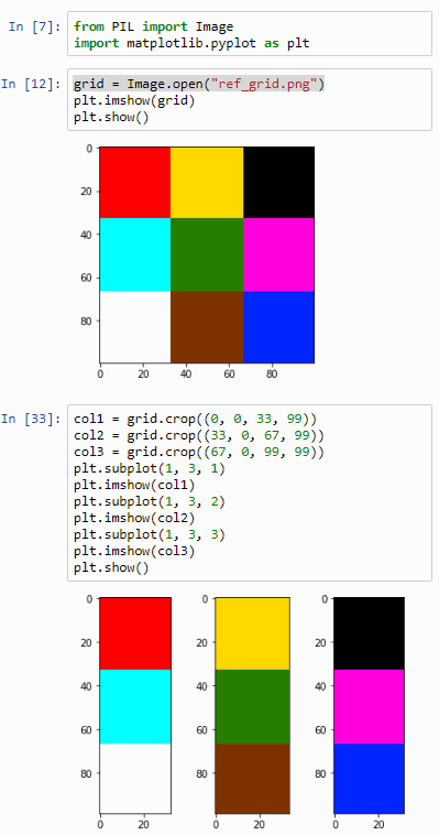
Let’s go back to the original image shown with this post: it’s a 100 x 100 pixel image, purposefully and deliberately divided in a 3 x 3 grid. Why? Because 100 isn’t divided by 3. So:

• in the corners, we have 33 x 33 pixels squares,
• in the center we have a 34 x 34 pixels square,
• in the top and bottom center section we have two rectangles of 34 pixels wide and 33 pixels tall,
• In the left and right section of the middle band of the image we have two rectangles of 33 pixels wide and 34 pixels tall.

What’s the importance of this image? It allows us to experiment in a convenient way with cropping. See, when dealing with array data it’s very easy to be just one-element off. You forget to process the last or first element, your offset is just one-off, or another couple of hundred variations on this basic scenario.

Let’s start by cutting the image into strips:

from PIL import Image
import matplotlib.pyplot as plt

grid = Image.open("ref_grid.png")
col1 = grid.crop((0, 0, 33, 99))
col2 = grid.crop((33, 0, 67, 99))
col3 = grid.crop((67, 0, 99, 99))

plt.subplot(1, 3, 1)
plt.imshow(col1)
plt.subplot(1, 3, 2)
plt.imshow(col2)
plt.subplot(1, 3, 3)
plt.imshow(col3)

plt.show()

The output of this script is as follows:

Now let’s see if we can loop this operation:

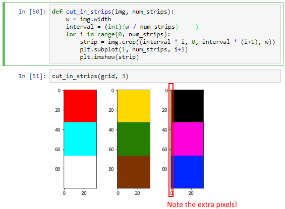
def cut_in_strips(img, num_strips):
    w = img.width
    interval = w / num_strips
    for i in range(0, num_strips):
        strip = img.crop((interval * i, 0, interval * (i+1), w))
        plt.subplot(1, num_strips, i+1)
        plt.imshow(strip)

cut_in_strips(grid, 3)

It works, but we actually sort of got lucky here. The key is that the width of our image is 100 pixels, and 100 doesn’t divide exactly by 3. It turns out that when we calculate interval, the variable automatically assuming the floating point data type. This may not always be the case (and certainly not in all languages). We can actually simulate what could go wrong by forcing interval into an integer datatype:

interval = (int)(w / num_strips)

You can see now that the third strip shows an extra pixel-edge that is clearly overflow from the third one.

“What’s the big deal?”, you might ask. After all, Python got it right the first time. Why bother?

Because Python might not get it right all the time. Our explicit conversion to int raises a typical off-by-one error. Furthermore: as images are typically converted to 2-dimensional arrays, and as we can have hundreds of tiles next to each other, this kind of one-off errors can easily snowball into big problems.

And in defense of sell-documenting code, the correct syntax to calculate the interval statement should be something more along the lines of:

interval = (float)(w * 1.0 / num_strips)

Remember, the ultimate goal is to break apart a “native” 500 x 500 Pathomation time into smaller pieces (say 25 100 x 100 tiles) and be able to parallelize tasks on these smaller tasks (as well as operate at a coarser zoomlevel).

So with this in mind, we can now plot any image into an arbitrary grid of images:

def plot_as_grid(img, num_rows, num_cols):
    w = img.width
    h = img.height
    interval_x = (float)(w * 1.0 / num_cols)
    interval_y = (float)(h * 1.0 / num_rows)
    for y in range(0, num_rows):
        for x in range(0, num_cols):
            cell = img.crop((interval_x * x, interval_y * y, interval_x * (x+1), interval_y * (y + 1)))
            plt.subplot(num_rows, num_cols, y * num_cols + x + 1)
            plt.imshow(cell)

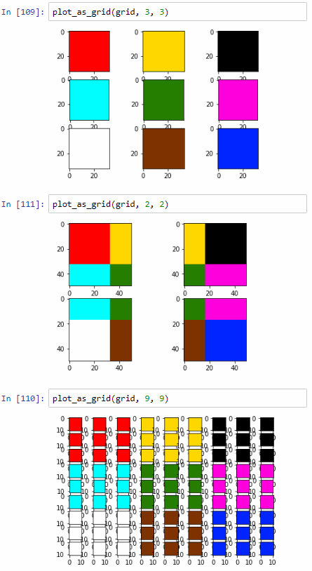
plot_as_grid(grid, 3, 3)
plot_as_grid(grid, 2, 2)
plot_as_grid(grid, 9, 9)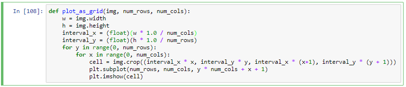

 Re-constituting an image