In our latest article we discussed how Pathomation works with large enterprises and OEM vendors to continuously improve its SDK facilities and specific programming language support.
Once customers are satisfied with our interfaces, the next question usually is about scaling: they figured out how to programmatically convert a JSON file from an AI provider into WKT-formatted PMA.core annotations, but what if there are hundreds, thousands, or even hundreds of thousands of spots to identify on a slide?
First scalability checks
How do you even define scalability? Yes, everything must always be able to handle more stuff in less time. That’s rather vague…
Visiting conferences helped us in this regard: looking around, we discovered sample data sets that others were using for validation and stress testing. One such dataset is published through a Nature paper on cell segmentation. We also refer to this dataset in our Annotations et al article.
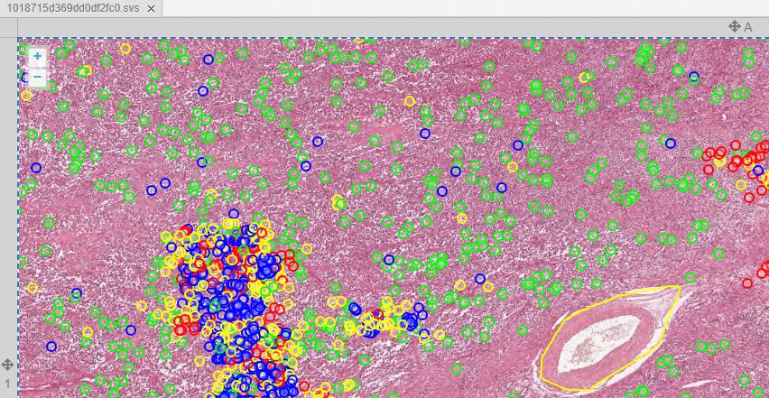
We obtained the code from https://github.com/DeepPathology/MITOS_WSI_CCMCT and got to work, scripting the conversion from the native (SQLite) format to records in our own (Microsoft SQLServer) database. 750,000 records were processed this way. A snapshot of just one slide is shown below in PMA.studio:
We admit we cheated to do the original import: Back in 2016, we didn’t have all the necessary and flexible API calls in PMA.core yet, let alone the convenient SDK interfaces for Python, PHP, and Java. So we used a custom script that translated the native records from the Nature paper into direct SQL statements. Not for the faint of heart, and only possible because we understand our own database structure in detail.
This initial experiment dates back a few years ago already (2016!). Today, you would solve this kind of problem through an ELT or ETL pipeline in an environment like Microsoft Azure Data Factory.
A more systematic approach
Fast-forward to last year. In 2022, we published a series of articles on software validation. Initial user acceptance testing – UAT – focuses on functionality however rather than scalability.
Can we exploit this mechanism to examine scalability as well? Or at least keep an eye on performance?
The way our approach works: we write out a User Requirement Specification – URS – that then gets its own UAT. The UAT is a Python Jupyter Notebook (using PMA.python) script. This script consists of different blocks that can be executed independently of each other.
The different kinds of annotations and how these translate to WKT-strings (as stored in our database) is described in a recent article on PMA.studio. The corollary for testing means that each cell in the Jupyter Notebook can test one specific type of annotation.
Linear scaling
Our first extension involved writing loops around our already in place test-code for the various types of annotations. The question we’re effectively asking: if it takes x amount of time to store a single annotation of type y; does it take n * x amounts of time to store n annotations?
The test results below suggest it does:
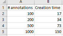
We were really excited with the results achieved. Our data shows that creating new annotations is a linear process: registering 1000 annotations takes roughly 10 times longer than registering 100 annotations. Inserting the 1000th annotation takes the same amount of time as inserting the 1st, 100th, 200th, or 500th annotation.
Loading and rendering considerations
Storing and retrieving data are different operations.
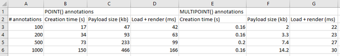
Our original data shows the times needed to create annotations. Luckily, it doesn’t take nowhere nearly as long to load and render annotations. But it still has some impact: more annotations will impact loading (and rendering) times in environments like PMA.studio. Below are the payload sizes and loading times of the same annotations we just created:
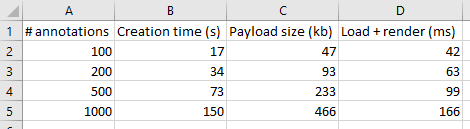
The conclusion from the table is that while 1000 annotations take 10 times longer to generate, and are 10 times larger in payload, they only take 4 times longer to load and render. That’s good!
But at the same time there is clearly a (albeit explainable) performance degradation as the annotation payload for a slide increases.
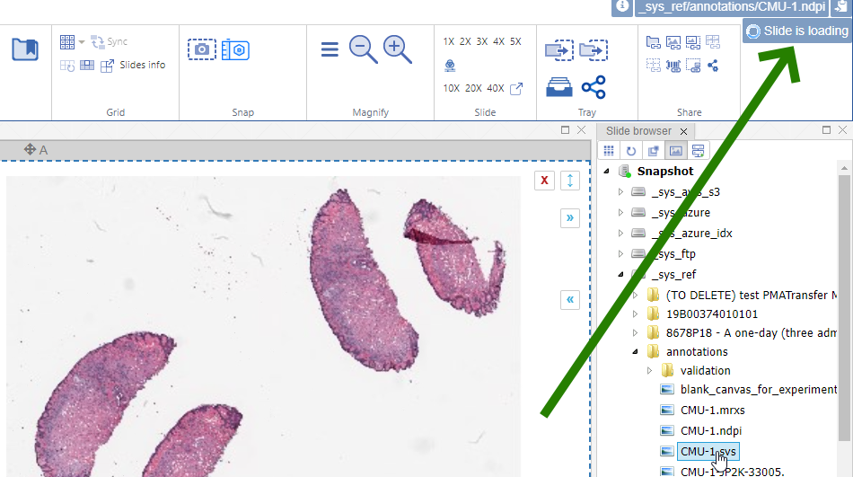
This is where user feedback becomes important, as well as (user) expectation management. A “slide loading” event can result in visual feedback like a spinning wheel cursor. In PMA.studio this is tackled by a status update in the top-right corner of the interface.
Keep in mind that the tests described here are performed in Jupyter notebooks. When we open one of the mitosis slides with real-world annotations, we find that it takes 9 seconds to load an annotation payload of 6.1 MB. The slide in question contains 13,781 annotations.
A better mousetrap for many landmark annotations
Our examples in the paragraph above indicate that we’re going to get into trouble with real-world datasets. We estimate that when, doing whole slide image analysis for something as mundane as a Ki67 marker (e.g. through interfacing with an external AI provider), we end up with anywhere between 100,000 and 200,000 individual cells, and therefore landmark annotations in PMA.core and PMA.studio. Extrapolating our earlier findings; it would take over 40 seconds to load these (and a payload of 4 MB)!
A MULTIPOINT annotation provides an alternative over individual POINT annotations then. Think of a multipoint annotation as a polygon, but without the lines. You can also think of these as a disconnected graph with only vertices and no edges.
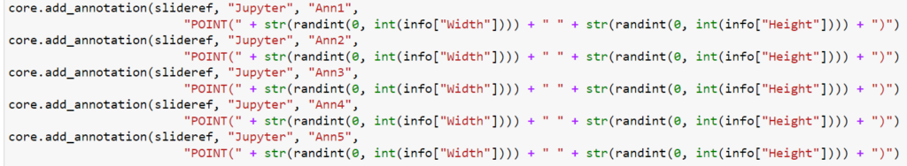
Let’s start with a simple example: let’s create 5 landmark annotations on a slide, by placing individual POINT annotations on them:
Let’s do the same via a MULTIPOINT annotation:
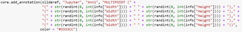
Even if you don’t read Python code, you can still see that the POINT annotations require the creation of five (5) annotations, whereas the MULTIPOINT annotation only requires one. Consequently, the first code snippet takes 0.71 seconds to execute; the second one only 0.14.
MULTIPOINT annotations are therefore the preferred way to go when you have a lot of individual cells to annotate. This is how the results compare to our original tests:
You can get more technical (WKT syntax) related information on MULTIPOINT annotations here. When working a lot with WKT annotations in Python, it may also be worthwhile to have a look at the Shapely library for easier syntax handling.
Current challenges (opportunities)
In some cases, MULTIPOINTs may become so dense that an actual density-map becomes more useful. Creating and handling those is a topic for a future blog article.
Including said heatmaps, in this article we pointed at three different way to handle landmark annotations. What you end up using though, is up to you, and will depend on your unique needs. There’s no one size fits all.
With such a big difference in performance, why would you ever want to use POINT annotations in the first place? Here are a couple of reasons:
- Your annotations are subject to review and need to be able to be modified if needed; we currently don’t have a good way of doing this yet for MULTIPOINT annotations.
- As a MULTIPOINT annotation is only one annotation, it is bound to a single classification, too. If you have MANY annotation classes with only a couple of points into each one, then individual POINT annotations may still be the way to go.
- Your annotations are created over time, by different users (or algorithms). If the landmark build up gradually, switching between different MULTIPOINT annotations may result in a very confusing end-user experience. This in turn can be resolved however by deleting the original MULTIPOINT annotation and overriding it with a newer more complex WKT-string as time proceeds.
Where to go next?
We’re constantly striving to make our software (both the PMA.core tile server and the PMA.studio cockpit environment) more flexible, powerful, and generally fit for the widest variety of use cases possible.
We don’t know what we don’t know yet though. Interesting new applications crop up in labs around the world every day. Have a scenario that you’re not seeing on our blog? Let us know, and let’s collaborate on making optimal analytical content delivery a reality.