Update on testing

A performance conundrum

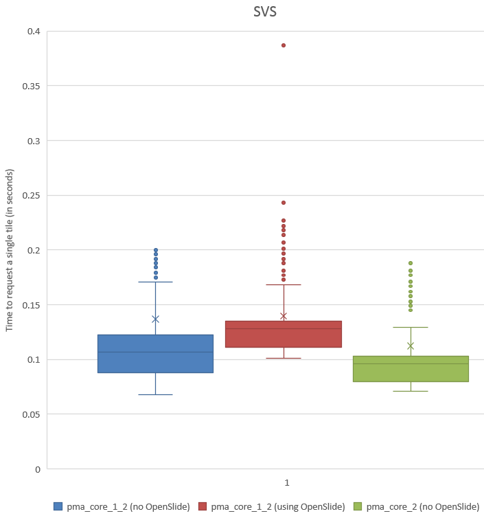
In a previous blog post, we showed how our own software compares to the legacy OpenSlide library. We explained our testing strategy, and did a statistical analysis of the file formats. We analyzed the obtained data for two out of five common WSI file formats.

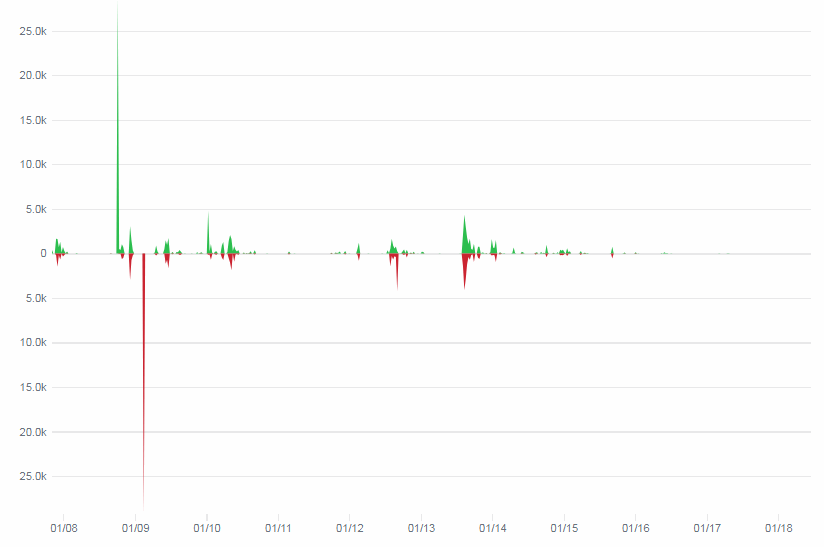
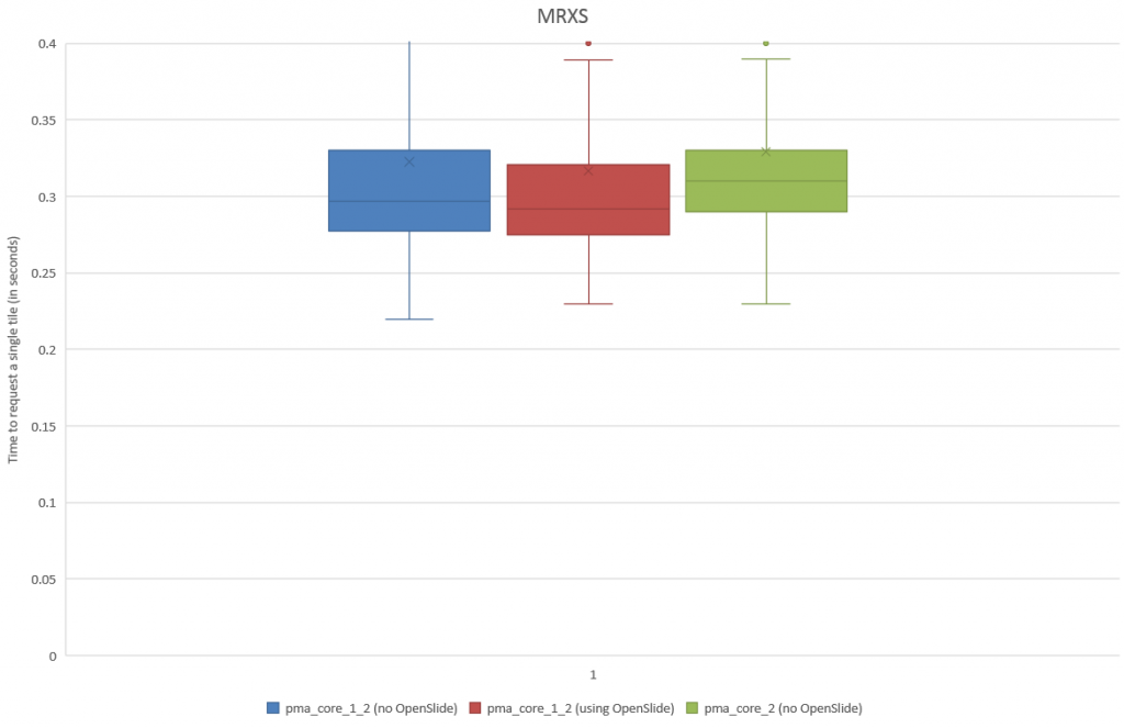
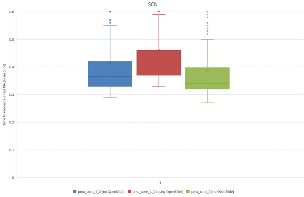
We subsequently ran the tests for three more formats, but ended up with somewhat of a conundrum. Below are the box and whisker plots for the Leica SCN file format, as well as the 3DHistech MRXS file format. The chart suggests OpenSlide is far superior.

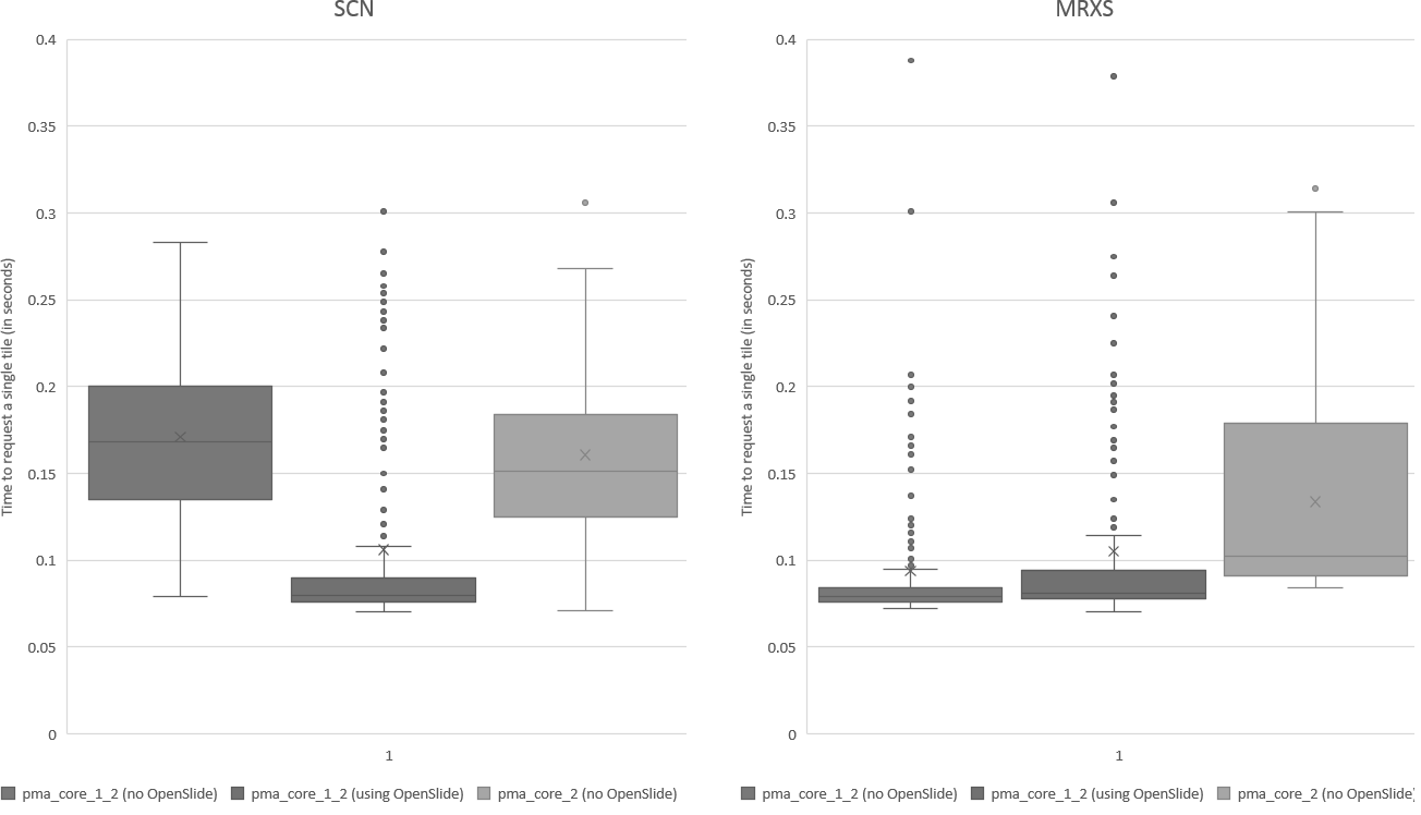
The differences are clear; but at the time so outspoken, that it was unlikely just due to the implementation, especially in light of our results. Case in point: the SCN file format differs little from the SVS format (they’re move adapted and renamed variants of the generic TIFF format).

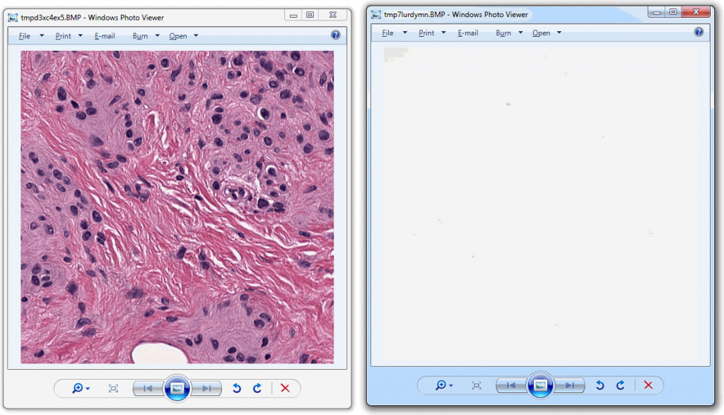
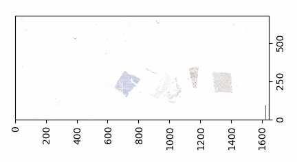
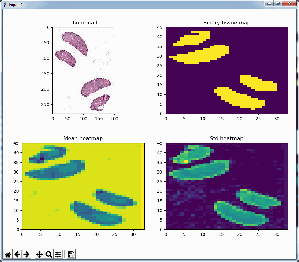
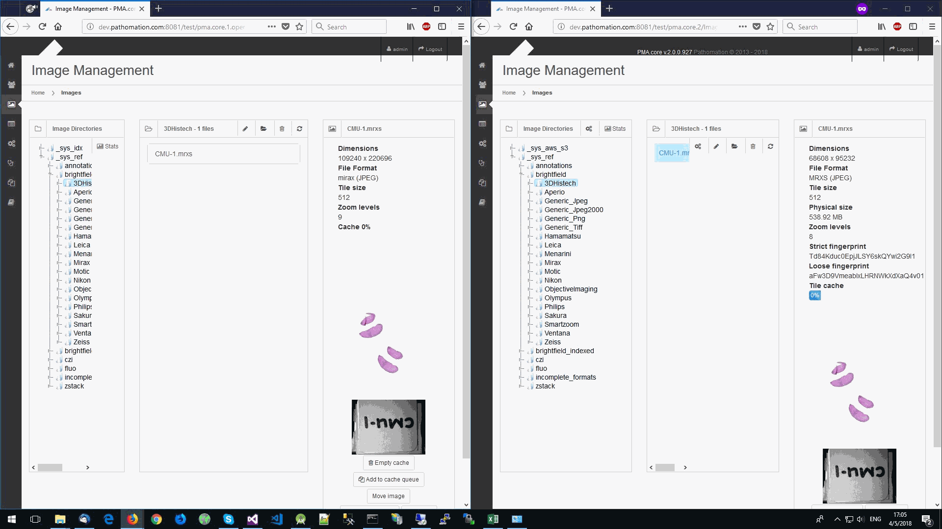
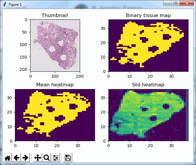
So we started looking at a higher level of the SCN file that we were using for our analysis. Showing the slide’s meta-data in PMA.core 1, PMA.core 1 + OpenSlide, and PMA.core 2. As PMA.core 1 and PMA.core 2 show similar performance, we only include PMA.core 2 (on the right) in the screenshot below.

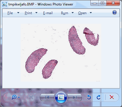
What happens is that PMA.core 2 only identifies the tissue on the glass, while OpenSlide not only identifies the tissue, but also builds a virtual whitespace area around the slide. This representation of the slide in OpenSlide is therefore much larger than the representation of slide in PMA.core (even though we’re talking about the same slide). The pixel space is with OpenSlide is almost 6 times bigger (5.76 times to be exact); but all of that extra space are just empty tiles.

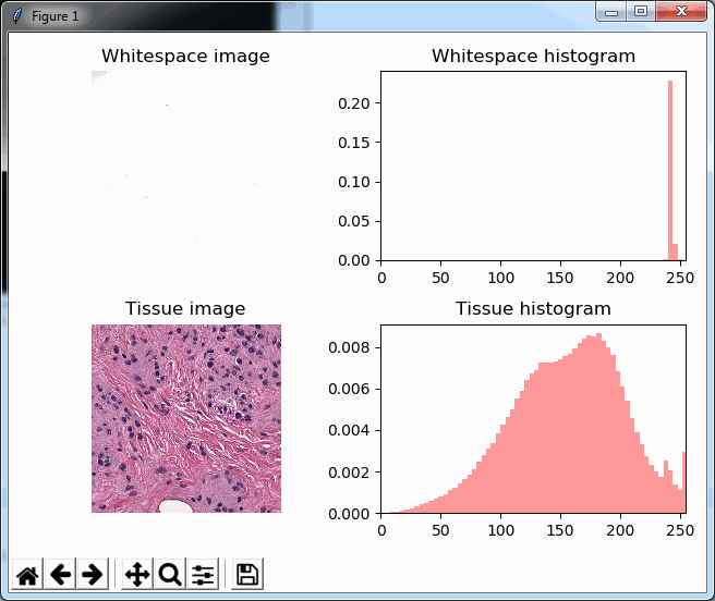
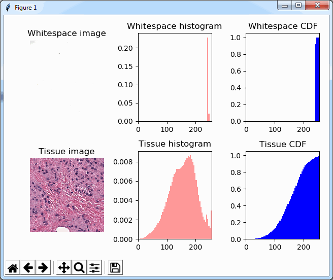
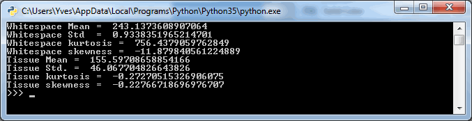
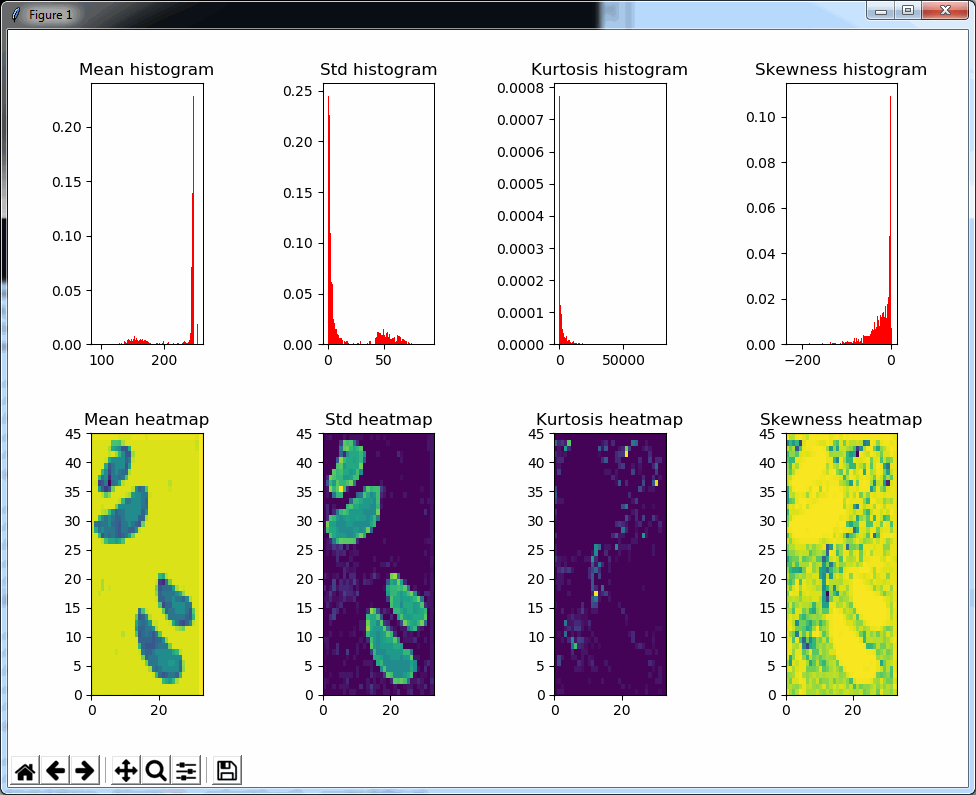
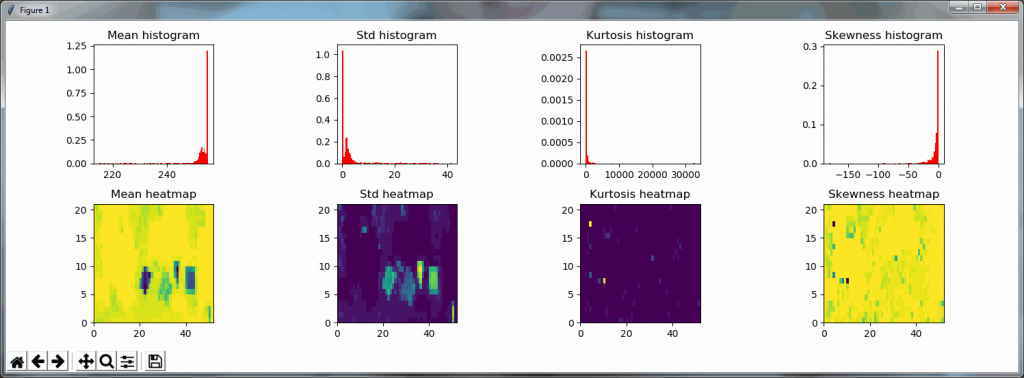
Now when we’re doing random sampling of tiles, we select from the entire pixel space. So, by chance, when selecting random tiles from the OpenSlide rendering engine, we’re much more likely to end up with an empty tile, than with PMA.core. Tiles get send back to the client in JPEG files, and blank tiles can be compressed and reduced in size much more than actual tissue tiles. We looked at the histogram and cumulative frequency distribution of pixel values in our latest post.

The same logic applies to the MRXS format: A side by side comparison also reveals that the pixel space in the OpenSlide build is much larger than in PMA.core.

The increased chance of ending up with a blank tile instead of real tissue doesn’t just explain the difference in mean retrieval times, it also explains the difference in variance that can be seen in the box and whisker plots.

Is_tissue() to the rescue

But wait, we just wrote that is_tissue() function earlier, that let’s us detect whether an obtained tile is blank or has tissue in it, right? Let’s use that one to see if a tile is whitespace or tissue. If it is tissue, we count the result in our statistic, it it’s not, we leave it out, and continue until we do hit a tissue tile that is worthy of inclusion.

To recap, here’s the code to our is_tissue() function (which we can’t condone for general use, but it’s good enough to get the job done here):

def is_tissue(tile):
    pixels = np.array(tile).flatten()        # np refers to numpy
    mean_threahold = np.mean(pixels) < 192   # 75th percentile
    std_threshold = np.std(pixels) < 75
    return mean_threahold == True and std_threshold == True

And our code for tile retrieval becomes like this:

def get_tiles(server, user, pwd, slide, num_trials = 100):
    session_id = pma.connect(server, user, pwd)
    print ("Obtained Session ID: ", session_id)
    info = pma.get_slide_info(slide, session_id)
    timepoints = []
    zl = pma.get_max_zoomlevel(slide, session_id)
    print("\t+getting random tiles from zoomlevel ", zl)
    (xtiles, ytiles, _) = pma.get_zoomlevels_dict(slide, session_id)[zl]
    total_tiles_requested = 0
    while len(timepoints) <= num_trials:
        xtile = randint(0, xtiles)
        ytile = randint(0, ytiles)
        print ("\t+getting tile ", len(timepoints), ":", xtile, ytile)
        s_time = datetime.datetime.now()    # start_time
        tile = pma.get_tile(slide, xtile + x, ytile + y, zl, session_id)
        total_tiles_requested = total_tiles_requested + 1
        if is_tissue(tile):
            timepoints.append((datetime.datetime.now() - s_time).total_seconds())
    pma.disconnect(session_id)
    print(total_tiles_requested, “ number of total tiles requested”)
    return timepoints

Note that at the end of our test function, we print out how many tiles we actually had to retrieve from each slide, in order to reach a sampling size that matches the trial_size parameter.

Running this on the MRXS sample both in our OpenSlide build and PMA.core 2 confirms our hypothesis about the increase in pixel space (and a bias for empty tiles). In our OpenSlide build, we have to weed through 4200 tiles to get a sample of 200 tissue tiles; in PMA.core 2 we “only” require 978 iterations.

Plotting the results as a box and whisker chart, we now get:

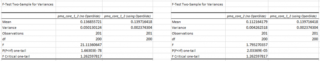
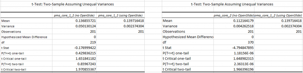
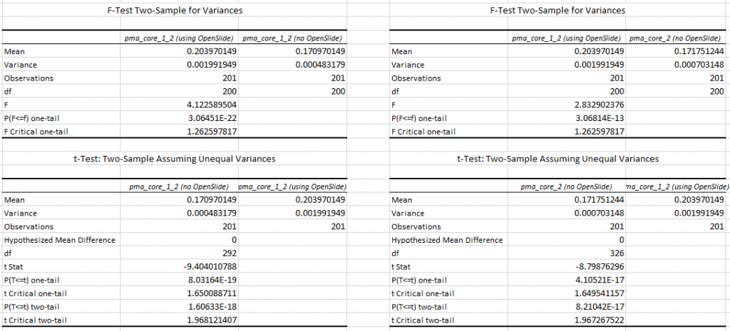
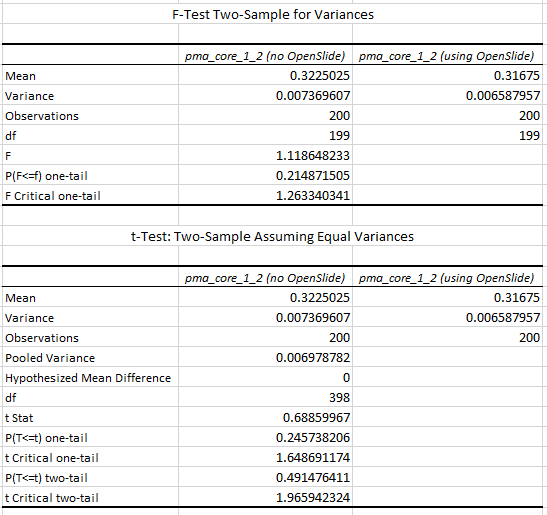
We turn to statistics once again to support our hypothesis:

We can do the same for SCN now. First, let’s see if we can indeed use the Is_Tissue() function to on the slide as a filter:

This looks good, and we run the same script as earlier. We notice the same discrepancy of overrepresented blank tiles in the SCN file when using OpenSlide. In our OpenSlide build, we have to retrieve 3111 tiles. Using our own implementation, only 563 tiles are needed.

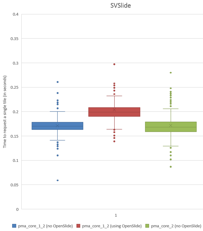
When we do a box and whisker plot, we confirm the superior performance of PMA.core compared to OpenSlide:

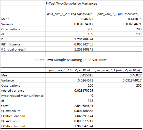
The statistics further confirm the observations of the box and whisker plot (p-value of 0.004 when examining the difference in means):

What does it all mean?

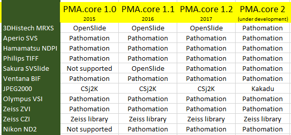
We generated all of the above and previous statistics and test suites to confirm that our technology is indeed faster than the legacy OpenSlide library. We did this on three different versions of PMA.core: version 1.2, a custom build of version 1.2 using OpenSlide where possible, and PMA.core 2.0 (currently under development). We can summarize our findings like this:

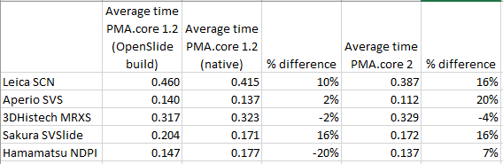
Note that we had to modify our testing strategy slightly for MRXS and SCN. The table doesn’t really suggest that it takes twice as long to read an SCN file compare to an SVSlide file. The discrepancies between the different file formats is the result of selecting either only tissue slides (MRXS, SCN), or a random mixture of both tissue and blank tiles.

When requesting tiles in a sequential manner (we’ll come back to parallel data retrieval in the future), the big takeaway number is that PMA.core is on average 11% faster than OpenSlide.


Dude, where’s my tissue?

Whitespace and tissue

Let’s say that you have a great algorithms to distinguish between PDL1- and a CD8-stained cells.

Your first challenge to run this on real data, is to find the actual tiles that contain tissue, rather than just whitespace. This is because your algorithm might be computationally expensive, and therefore you want to run it only on parts of the slide where it makes sense to do the analysis. In order words: you want to eliminate the whitespace.

At our PMA.start website, you can find OpenCV code that automatically outlines an area of tissue on a slide, but in this post we want to tackle things at a somewhat more fundamental level.

Let’s see if we can figure out a mechanism ourselves to distinguish tissue from whitespace.

First, we need to do some empirical exploration. So let’s start by downloading a reference slide from OpenSlide and request its thumbnail through PMA.start:

from pma_python import core
slide = "C:/my_slides/CMU-1.svs"
core.get_thumbnail_image(slide).show()

As we can see, there’s plenty of whitespace to go around. Let’s get a whitespace tile at position (0,0), and a tissue tile at position (max_x / 4, max_y / 2). Intuitively you may want to go for (max_x/2, max_y/2), but that wouldn’t get us anywhere here. So pulling up the thumbnail first is important for this exercise, should you do this on a slide of your own (and your coordinates may vary from ours).

Displaying these tiles two example tiles side by side goes like this:

from pma_python import core
slide = "C:/my_slides/CMU-1.svs"
max_zl = core.get_max_zoomlevel(slide)
dims = core.get_zoomlevels_dict(slide)[max_zl]

tile_0_0 = core.get_tile(slide, x=0, y=0, zoomlevel=max_zl)
tile_0_0.show()

tile_x_y = core.get_tile(slide, x=int(dims[0] / 4), y=int(dims[1] / 2), zoomlevel=max_zl)
tile_x_y.show()

And looks like this:

Now that we have the two distinctive tiles, let’s convert both to grayscale and add a histogram to our script for each:

from pma_python import core
import matplotlib.pyplot as plt
import numpy as np

slide = "C:/my_slides/CMU-1.svs"
max_zl = core.get_max_zoomlevel(slide)
dims = core.get_zoomlevels_dict(slide)[max_zl]

# obtain whitespace tile
tile_0_0 = core.get_tile(slide, x=0, y=0, zoomlevel=max_zl)
# Flatten the whitespace into 1 dimension: pixels
pixels_0_0 = np.array(tile_0_0).flatten()

# obtain tissue tile
tile_x_y = core.get_tile(slide, x=int(dims[0] / 4), y=int(dims[1] / 2), zoomlevel=max_zl)
# Flatten the tissue into 1 dimension: pixels
pixels_x_y = np.array(tile_x_y).flatten()

# Display whitespace image
plt.subplot(2,2,1)
plt.title('Whitespace image')
plt.axis('off')
plt.imshow(tile_0_0, cmap="gray")

# Display a histogram of whitespace pixels
plt.subplot(2,2,2)
plt.xlim((0,255))
plt.title('Whitespace histogram')
plt.hist(pixels_0_0, bins=64, range=(0,256), color="red", alpha=0.4, normed=True)

# Display tissue image
plt.subplot(2,2,3)
plt.title('Tissue image')
plt.axis('off')
plt.imshow(tile_x_y, cmap="gray")

# Display a histogram of whitespace pixels
plt.subplot(2,2,4)
plt.xlim((0,255))
plt.title('Tissue histogram')
plt.hist(pixels_x_y, bins=64, range=(0,256), color="red", alpha=0.4, normed=True)

# Display the plot
plt.tight_layout()
plt.show()

As you can see, we make use of PyPlot subplots here. The output looks as follows, and shows how distinctive the histogram for whitespace is compared to actual tissue areas.

We can add a cumulative distribution function to further illustrate the difference:

# Display whitespace image
plt.subplot(2,3,1)
plt.title('Whitespace image')
plt.axis('off')
plt.imshow(tile_0_0, cmap="gray")

# Display a histogram of whitespace pixels
plt.subplot(2,3,2)
plt.xlim((0,255))
plt.title('Whitespace histogram')
plt.hist(pixels_0_0, bins=64, range=(0,256), color="red", alpha=0.4, normed=True)

# Display a cumulative histogram of the whitespace
plt.subplot(2,3,3)
plt.hist(pixels_0_0, bins=64, range=(0,256), normed=True, cumulative=True, color='blue')
plt.xlim((0,255))
plt.grid('off')
plt.title('Whitespace CDF')

# Display tissue image
plt.subplot(2,3,4)
plt.title('Tissue image')
plt.axis('off')
plt.imshow(tile_x_y, cmap="gray")

# Display a histogram of whitespace pixels
plt.subplot(2,3,5)
plt.xlim((0,255))
plt.title('Tissue histogram')
plt.hist(pixels_x_y, bins=64, range=(0,256), color="red", alpha=0.4, normed=True)

# Display a cumulative histogram of the tissue
plt.subplot(2,3,6)
plt.hist(pixels_x_y, bins=64, range=(0,256), normed=True, cumulative=True, color='blue')
plt.xlim((0,255))
plt.grid('off')
plt.title('Tissue CDF')

Note that we’re now using a 2 x 3 grid to display the histogram and the cumulative distribution function (CDF) next to each other, which ends up looking like this:

Back to basic (statistics)

We could now write a complicated method that manually scans through the pixel-arrays and assesses how many bins there are, how they are distributed etc. However, it is worth noting that the histogram-buckets that are NOT showing any values in the histogram, are not pixels-values of 0; the histogram shows a frequency, therefore, empty spaces in the histogram simply means that NO pixels are available at a given intensity.

So after we visualized the pixel distribution through MatPlotLib’s PyPlot, it’s worth looking as some basic statistics for the flattened pixels arrays. Numpy’s basic .std() and .mean() functions are good enough to do the job for now. The script becomes:

from pma_python import core
import matplotlib.pyplot as plt
import numpy as np
import scipy.stats

slide = "C:/my_slides/CMU-1.svs"
max_zl = core.get_max_zoomlevel(slide)
dims = core.get_zoomlevels_dict(slide)[max_zl]

# obtain whitespace tile
tile_0_0 = core.get_tile(slide, x=0, y=0, zoomlevel=max_zl)
# Flatten the whitespace into 1 dimension: pixels
pixels_0_0 = np.array(tile_0_0).flatten()
# print whitespace statistics
print("Whitespace Mean = ", np.mean(pixels_0_0))
print("Whitespace Std  = ", np.std(pixels_0_0))
print("Whitespace kurtosis = ", scipy.stats.kurtosis(pixels_0_0))
print("Whitespace skewness = ", scipy.stats.skew(pixels_0_0))

# obtain tissue tile
tile_x_y = core.get_tile(slide, x=int(dims[0] / 4), y=int(dims[1] / 2), zoomlevel=max_zl)
# Flatten the tissue into 1 dimension: pixels
pixels_x_y = np.array(tile_x_y).flatten()
# print tissue statistics
print("Tissue Mean = ", np.mean(pixels_x_y))
print("Tissue Std. = ", np.std(pixels_x_y))
print("Tissue kurtosis = ", scipy.stats.kurtosis(pixels_x_y))
print("Tissue skewness = ", scipy.stats.skew(pixels_x_y))

The output (for the same tiles as we visualized using PyPlot earlier is as follows:

The numbers suggest that the mean-(grayscale-)value of a Whitespace tile is a lot higher than that of a tissue tile. More importantly: the standard deviation (variance squared) could be an even more important indicator. Naturally we would expect the standard deviation of (homogenous) whitespace to be much less than that of tissue pictures containing a range of different features.

Kurtosis and skewness are harder to interpret and place, but let’s keep them in there for our further investigation below.

Another histogram

We started this post by analyzing an individual tile’s grayscale histogram. We now summarized that same histogram in a limited number of statistical measurements. In order to determine whether those statistical calculations are an accurate substitute for a visual inspection, we compute those parameters for each tile at a zoomlevel, and then plot those data as a heatmap.

The script for this is as follows. Depending on your fast your machine is, you can play w/ the zoomlevel parameter at the top of the script, or set it to the maximum zoomlevel (at which point you’ll be evaluating every pixel in the slide.

from pma_python import core
import matplotlib.pyplot as plt
import numpy as np
import scipy.stats
import sys

slide = "C:/my_slides/CMU-1.svs"
max_zl = 6 # or set to core.get_max_zoomlevel(slide)
dims = core.get_zoomlevels_dict(slide)[max_zl]

means = []
stds = []
kurts = []
skews = []

for x in range(0, dims[0]):
    for y in range(0, dims[1]):
        tile = core.get_tile(slide, x=x, y=y, zoomlevel=max_zl)
        pixels = np.array(tile).flatten()
        means.append(np.mean(pixels))
        stds.append(np.std(pixels))
        kurts.append(scipy.stats.kurtosis(pixels))
        skews.append(scipy.stats.skew(pixels))
    print(".", end="")
    sys.stdout.flush()
print()

means_hm = np.array(means).reshape(dims[0],dims[1])
stds_hm = np.array(stds).reshape(dims[0],dims[1])
kurts_hm = np.array(kurts).reshape(dims[0],dims[1])
skews_hm = np.array(skews).reshape(dims[0],dims[1])

plt.subplot(2,4,1)
plt.title('Mean histogram')
plt.hist(means, bins=100, color="red", normed=True)
plt.subplot(2,4,5)
plt.title('Mean heatmap')
plt.pcolor(means_hm)

plt.subplot(2,4,2)
plt.title('Std histogram')
plt.hist(stds, bins=100, color="red", normed=True)
plt.subplot(2,4,6)
plt.title("Std heatmap")
plt.pcolor(stds_hm)

plt.subplot(2,4,3)
plt.title('Kurtosis histogram')
plt.hist(kurts, bins=100, color="red", normed=True)
plt.subplot(2,4,7)
plt.title("Kurtosis heatmap")
plt.pcolor(kurts_hm)

plt.subplot(2,4,4)
plt.title('Skewness histogram')
plt.hist(skews, bins=100, color="red", normed=True)
plt.subplot(2,4,8)
plt.title("Skewness heatmap")
plt.pcolor(skews_hm)

plt.tight_layout()
plt.show()

The result is a 2 row x 4 columns PyPlot grid, shown below for a selected zoomlevel of 6:

The standard deviation as well as the mean grayscale value of a tile seem accurate indicators to determine the position of where tissue can be found on the slide; skewness and kurtosis not so much.

Both the mean histogram and the standard deviation histogram show a bimodal distribution, and we can confirm their behavior by looking at other slides. It even works on slides that are only lightly stained (we will return to these at a later post and see how we can make the detection better in these:

A binary map

We can now write a function that determines whether a tile is (mostly) tissue, based on the mean and standard deviation of the grayscale pixel values, like this:

def is_tissue(tile):
    pixels = np.array(tile).flatten()
    mean_threahold = np.mean(pixels) < 192   # 75th percentile
    std_threshold = np.std(pixels) < 75
    return mean_threahold == True and std_threshold == True

Writing a similar function that determines whether a tile is (mostly) whitespace, is possible, too, of course:

def is_whitespace(tile):
    return not is_tissue(tile)

Similarly, we can even use this function to now construct a black and white map of where the tissue is located on a slide. The default color map of PyPlot on our system nevertheless rendered the map blue and yellow:

In closing

This post started with “Let’s say that you have a great algorithms to distinguish between PDL1- and a CD8-stained cells.”. We didn’t quite solve that challenge yet. But we did show you some important initial steps you’ll have to take to get to that part eventually.

In the next couple of blogs we want to elaborate on the topic of tissue detection some more. We want to discuss different types of input material, as well as see if we can use a machine learning classifier to replace the deterministic mapping procedure developed here.

But first, we’ll get back to testing, and we’ll tell you why it was important to have the is_tissue() function from the last paragraph developed first.

To OpenSlide or not to OpenSlide

The legacy

When you say digital pathology or whole slide imaging, sooner or later you end up with OpenSlide. This is essentially a programming library. Back in 2012, a pathologist alerted me to it (there’s some irony to the fact that he found it before me, the bioinformatician). He didn’t know what to do with it, but it looked interesting to him.

OpenSlide is how Pathomation got started. We actually contributed to the project.

We also submitted sample files to add to their public repository (and today, we use this repository frequently ourselves, as do many others, I’m sure).

Our names are mentioned in the Acknowledgements section of the OpenSlide paper.

But today, the project has rather slowed down. This is easy to track through their GitHub activity page:

Kudos to the team; they do still make an effort to fix bugs that crop up, today’s but activities seem limited to maintenance. Of course there’s a possibility that nobody gets the code through GitHub anymore, but rather through one of the affiliate projects that they are embedded into.

Consider this though: OpenSlide Discussions about supporting support for (immuno)fluorescence and z-stacking date back to 2012  , but never resulted in anything. Similarly, there are probably about a dozen file formats out there that they don’t support (or flavors that they don’t support, like Sakura’s SVSlide format, which was recently redesigned). We made a table of the formats that we support, and they don’t, at http://free.pathomation.com/pma_start_omero_openslide/

Free at last

Our own software, we’re proud to say, is OpenSlide-free. PMA.start no longer ships with the OpenSlide binaries. The evolution our software has gone through then is as follows (the table doesn’t list all the formats we support; for a full list see http://free.pathomation.com/formats):

At one time, we realized there was really only one file format left that we still ran through OpenSlide, and with the move to cloud storage (more on that in a later post), we decided we might as well make one final effort to re-implement a parser for 3DHistech MRXS slides ourselves.

Profiling

Of course all of this moving away from OpenSlide is useless if we don’t measure up in terms of performance.

So here’s what we did: we downloaded a number of reference slides from the OpenSlide website. Then, we took our latest GAMP5 validated version of our PMA.core 1.2 software, and rerouted it’s slide parsing routines to OpenSlide. This result in a PMA.core 1.2 build that instead of just 2 (Sakura SVSlide and 3DHistech MRXS), now reads 5 different WSI file formats through OpenSlide:  Sakura SVSlide, 3DHistech MRXS, Leica SCN, Aperio SVS, and Hamamatsu NDPI.

Our test methodology consist of the following steps:

For each slide:
    Determine the deepest zoomlevel
    From this zoomlevel select 200 random tiles
    Retrieve each tile sequentially
    Keep track of how long it takes to retrieve each tiles

We run this scenario of 3 instances of PMA.core:

  •                 PMA.core 1.2 without OpenSlide (except for SVSlide and MRXS)
  •                 PMA.core 1.2 custom-build with OpenSlide (for all 5 file formats)
  •                 PMA.core 2 beta without OpenSlide

The random tiles selected from the respective slides are different each time. The tiles extracted from slide.ext on PMA.core instance 1 are different from the ones retrieved through PMA.core instance 2.

Results

As simple as the above script sounds, we discovered some oddities while running them for each file format.

Let’s start w/ the two easiest to explain ones: SVS and SVSlide.

A histogram of the recorded times for SVSlide yields the following chart:

We can see visually that PMA.core 1.2 without OpenSlide is a little faster than the PMA.core 1.2 custom-build with OpenSlide, and that we were able to improve this performance yet again in PMA.core 2.

The p-value confirm this. First we do an F-test to determine what T-test we need (p-values of 1.66303E-78 and 2.03369E-05 suggests inequal variances),

Next, we find a p-value of 0.859 (n=200) for the difference in mean tile retrieval time between PMA.core 1.2 with and without OpenSlide, and a p-value of 2.363E-06 for the difference in means between PMA.core 1.2 with OpenSlide and PMA.core 2 without OpenSlide.

We see this as conclusive evidence that PMA.core 2 (as well as PMA.start, which contains a limited version of the PMA.core 2 code in the form of PMA.core.lite) can render tiles faster than OpenSlide can.

What about SVSlide?

Again, let’s start by looking at the histogram:

This is the same trend as we saw for SVS, so let’s see if we can confirm this with statistics. The F-statistic between PMA.core 1.2 with and without OpenSlide yields a p-value of 3.064E-22; between PMA.core 1.2 without OpenSlide and PMA.core 2 we get a p-value of 3.068E-13.

Subsequent T-tests (assuming unequal variance) between PMA.core 1.2 with and without OpenSlide show a p-value of  8.031E-19; between PMA.core 1.2 with OpenSlide and PMA.core 2 we get a p-value of 4.10521E-17 (one-tailed).

Again, we conclude that both PMA.core 1.2 and PMA.core 2 (as well as PMA.start) are faster to render Sakura SVSlide slides than OpenSlide.

What about the others?

We’re still working on getting data for the other file formats. Stay tuned!