Challenges and opportunities
It’s been well established that whole slide images are big. We wrote a tutorial on this ourselves.
This poses challenges for both computers and analysts alike:
Consider the pathologist that must identify x number of cells of a certain classification. How many should he aim for? How big should his field of view be to select from?…
Automation seems to be a solution, but here too limits crop up. Professional image analysis software is expensive, people need to be trained, and there are only so many pixels any GPU can process in any given time.
The solution comes in treating the image analysis process as a multi-phased project.
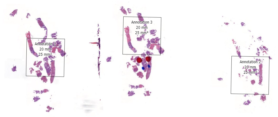
In the first phase, select fields of view and regions of interest can be prepared as annotations on top of a whole slide image. This pre-selection can be as simple as an automated algo that identifies entropy in a pixel environment, or a pathologist that carefully picks and curates regions of interest.
In other words: statistical (random) sampling is the name of the game. And our very own PMA.studio is a great solution to make these ground-truth annotations in.
Annotations in PMA.core
Whether via scripting or manual curation, annotations end up stored in PMA.core.
Internally, we store the annotations as Well-Known Text (WKT) strings, but they can be converted to several other file formats, too, including Excel CSV, Visiopharm MLD, Leica/Aperio XML, or Halo Annotation XML.
We provide several other resources regarding annotations that can provide more background:
- PMA.studio tutorial on how to make annotations
- PMA.UI tutorial on how to design custom annotation toolbars
- OpenCV tutorial on how to identify tissue regions in whole slide images
When your annotations are part of a random sampling exercise, chances are that you’re going to want to do more downstream operations with them.
In this article we will therefore:
- Use Jupyter and pma_python to interact with PMA.core
- Identify geometric (polygon) annotations and examine their properties
- Convert annotations to rectangular snapshots at high-resolution
- Save these extracted annotations as new separate high-resolution tiled TIFF slides
Core::get_annotations()
The Core module of our SDK contains a get_annotations() function already. Let’s start by examining what we get back when we invoke it on our sample slide:
from pma_python import core
core.connect("https://srv/pma.core/", "usr", "***")
slideref = "/rootdir/slide.mrxs"
annotations = core::get_annotations(slideref)
Now we can print the first element and see what it contains. We use the pprint library to make our output look pretty:
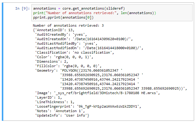
We can immediately see the audit trail, and beyond that the most obvious element is the Geometry. As you be deduced: the geometry defines all points that make up an annotation. In our case our polygon is merely a rectangle, so we find 5 (x, y) coordinates, with the fifth one being the same as the origin. The format can be generalized and written out in a symbolic annotation that looks like this:
POLYGON((x1 y1,x2 y2, x3 y3, x4 y4,…, xn yn,…, x1 y1))
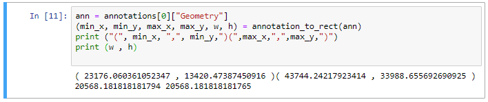
If we want to convert these annotations to snapshots, we need to determine the x y coordinates of the points that define a rectangle that contains all points of our original polygon.
In other words, for each of the x y pairs of coordinates given, we find the minimum and maximum x and y values. We can then use these to compute the width and height of the resulting (high resolution) snapshot.
Luckily this is easier to do than finding the largest rectangle within a polygon!
def annotation_to_rect(ann):
    points = ann.split(",")
    min_x = sys.maxsize
    max_x = sys.maxsize * -1
    min_y = sys.maxsize
    max_y = sys.maxsize * -1
    for point in points:
        (x, y) = point.split(" ")
        x = float(x)
        y = float(y)
        if x > max_x:
            max_x = x
        if x < min_x:
            min_x = x
        if y > max_y:
            max_y = y
        if y < min_y:
            min_y = y
    w = max_x - min_x
    h = max_y - min_y
    return (min_x, min_y, max_x, max_y, w, h)
And we can use this method to get the coordinates of the first annotation.
Core::get_region()
In earlier tutorials, we mostly stuck with extracting tiles from PMA.core. But if you want to extract arbitrary regions, you can use core::get_region() instead. The call uses the same coordinate system as used to store annotations.
Our next step then is to use these coordinates and parameters as arguments for the get_region() call.
region = core.get_region(slideref, min_x, min_y, w, h)
Without any additional parameters, get_region() automatically retrieves pixels at the deepest zoomlevel. While this is what you want, it is quite possible that your environment may be protected against such (perceived) over-zealous behavior and responds with an error:
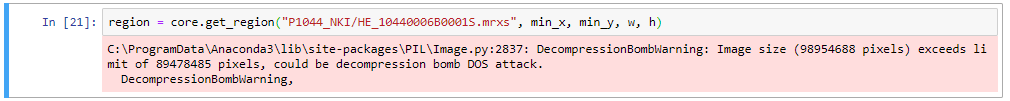
DOS attacks are a reasonable concern of course.
The solution then is to split up the coordinates in 4 quadrants. Like this:
region11 = core.get_region("slide.mrxs", min_x, min_y, w / 2, h / 2)
region12 = core.get_region("slide.mrxs", min_x + w/2, min_y, w / 2, h / 2)
region21 = core.get_region("slide.mrxs", min_x, min_y + h/2, w / 2, h / 2)
region22 = core.get_region("slide.mrxs", min_x + w/2, min_y + h/2, w / 2, h / 2)
Once the four quadrants are loaded, a new PIL image can be constructed, and the 4 quadrants can be pasted into the respective corners.
region_combo = Image.new('RGB', (int(math.ceil(w)), int(math.ceil(h))))
region_combo.paste(region11)
region_combo.paste(region12, (int(math.floor(w/2)), 0))
region_combo.paste(region21, (0, int(math.floor(h/2))))
region_combo.paste(region22, (int(math.floor(w/2)), int(math.floor(h/2))))
region_combo.save("region.jpg", "JPEG", quality = 95, optimize = True, progressive = True)
By working with quadrants, you’re effectively creating a de facto 2 x 2 grid. If this still doesn’t work for you, you can create 3 x 3 grids, or go even more refined.
Pyramidal TIFF
What’s missing? Say that your resulting extracted high-resolution snapshot is 8K x 5K pixels in size. You can work with that kind of image in some programs, but it’s not ideal. And your resulting snapshot can be even larger than that.
The solution is to not save your PIL image in a JPEG format. Instead, to save it as a pyramidal (tiled) TIFF. Some environments, like ASAP, even require this kind of input format.
After installing the gdal library, you can use the following method to convert any PIL image object into a pyramidal (tiled) TIFF:
def PILToTiff(pilref, output_file= "pil.tif", target_quality = 80, downscale_factor = 1):
    tileSize = 512
    tiff_drv = gdal.GetDriverByName("GTiff")
    output_filename =  output_file
    (w, h) = pilref.size
    ds = tiff_drv.Create(
        output_filename,  w,  h,  3,
        options=['BIGTIFF=YES',
            'COMPRESS=JPEG', 'TILED=YES', 'BLOCKXSIZE=' + str(tileSize), 'BLOCKYSIZE=' + str(tileSize),
            'JPEG_QUALITY=90', 'PHOTOMETRIC=RGB'
        ])

    tilesX = int(math.ceil(w / 512))
    tilesY = int(math.ceil(h / 512))
    totalTiles = tilesX * tilesY
    pbar = tqdm(total=totalTiles)
    for x in range(tilesX):
        for y in range(tilesY):
            pbar.update()

            x1 = x * 512
            y1 = y * 512
            x2 = min((x+1)*512, w)
            y2 = min((y+1)*512, h)

            tile = pilref.crop((x1, y1, x2, y2))
            arr = np.array(tile, np.uint8)

            # calculate startx starty pixel coordinates based on tile indexes (x,y)
            sx = x * tileSize
            sy = y * tileSize

            ds.GetRasterBand(1).WriteArray(arr[..., 0], sx, sy)
            ds.GetRasterBand(2).WriteArray(arr[..., 1], sx, sy)
            ds.GetRasterBand(3).WriteArray(arr[..., 2], sx, sy)

    pbar.close()
    ds.BuildOverviews('average', [pow(2, l) for l in range(1, 5)])
    ds = None
    print("Done; see result in ", output_filename)
When we now systematically want to convert all annotations from a set of slides into separate high-resolution pyramidal TIFF files, it’s just a matter of putting together the functions we’ve developed in this tutorial:
for slide in core.get_slides("/root_dir/path/…"):
    annotations = core.get_annotations(slide)
    ann_idx = 0
    for annotation in annotations:
        ann_img = AnnotationToPIL(slide, ann_idx)
        tif_file = "c:/output/" + os.path.basename(slide).replace(".", "_") + "_" + str(ann_idx) + ".tif"
        PILToTiff(ann_img, tif_file)
        ann_idx = ann_idx + 1
The result can be seen in PMA.start in the c:\output folder afterwards:
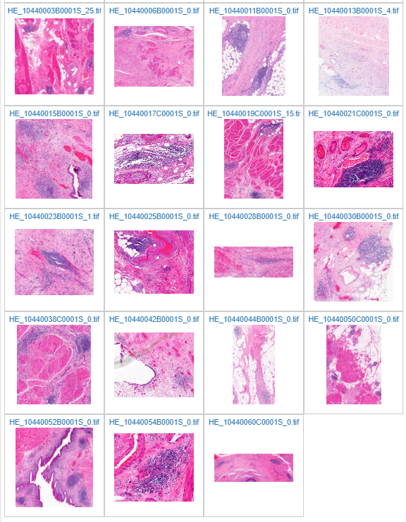
Ground truth
Image Analysis (IA) comes in many shapes: Artificial Intelligence (AI), Machine Learning (ML), Deep Learning (DL)… What they all need: curated data to train on. Sometimes it’s as simple as feeding them all the tiles contained in a whole slide image one by one, and we’ve done a couple of examples of this already on our blog.
At times however, supervised machine learning is the name of the game. For that, a pathologist may pre-select particularly interesting looking areas of interest. In other cases, statistical random sampling may help to make an existing algorithm more robust or fine-tune it.
The resulting regions of interest (whether manually annotated through PMA.studio or automated via an environment like OpenCV) can in turn be exported again in individual high-resolution images that represent true subsets of slides.
In this article, we showed how such a complete workflow can be facilitated by our very own PMA.python SDK. The resulting dataset is at the same high-resolution as the original, and the performance of the images is just as good as what you started with.
Of course you may not be using Python, or you may just be looking for something just a bit different. Need help? Do drop us a note. We love hearing about your use case, and think about how we can help solve problems.