Whitespace and tissue

Let’s say that you have a great algorithms to distinguish between PDL1- and a CD8-stained cells.

Your first challenge to run this on real data, is to find the actual tiles that contain tissue, rather than just whitespace. This is because your algorithm might be computationally expensive, and therefore you want to run it only on parts of the slide where it makes sense to do the analysis. In order words: you want to eliminate the whitespace.

At our PMA.start website, you can find OpenCV code that automatically outlines an area of tissue on a slide, but in this post we want to tackle things at a somewhat more fundamental level.

Let’s see if we can figure out a mechanism ourselves to distinguish tissue from whitespace.

First, we need to do some empirical exploration. So let’s start by downloading a reference slide from OpenSlide and request its thumbnail through PMA.start:

from pma_python import core
slide = "C:/my_slides/CMU-1.svs"
core.get_thumbnail_image(slide).show()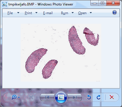

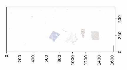
As we can see, there’s plenty of whitespace to go around. Let’s get a whitespace tile at position (0,0), and a tissue tile at position (max_x / 4, max_y / 2). Intuitively you may want to go for (max_x/2, max_y/2), but that wouldn’t get us anywhere here. So pulling up the thumbnail first is important for this exercise, should you do this on a slide of your own (and your coordinates may vary from ours).

Displaying these tiles two example tiles side by side goes like this:

from pma_python import core
slide = "C:/my_slides/CMU-1.svs"
max_zl = core.get_max_zoomlevel(slide)
dims = core.get_zoomlevels_dict(slide)[max_zl]

tile_0_0 = core.get_tile(slide, x=0, y=0, zoomlevel=max_zl)
tile_0_0.show()

tile_x_y = core.get_tile(slide, x=int(dims[0] / 4), y=int(dims[1] / 2), zoomlevel=max_zl)
tile_x_y.show()

And looks like this:

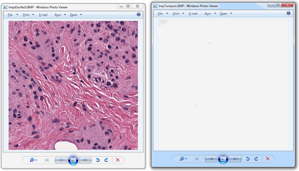
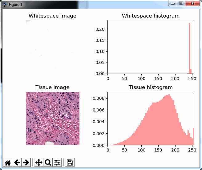
Now that we have the two distinctive tiles, let’s convert both to grayscale and add a histogram to our script for each:

from pma_python import core
import matplotlib.pyplot as plt
import numpy as np

slide = "C:/my_slides/CMU-1.svs"
max_zl = core.get_max_zoomlevel(slide)
dims = core.get_zoomlevels_dict(slide)[max_zl]

# obtain whitespace tile
tile_0_0 = core.get_tile(slide, x=0, y=0, zoomlevel=max_zl)
# Flatten the whitespace into 1 dimension: pixels
pixels_0_0 = np.array(tile_0_0).flatten()

# obtain tissue tile
tile_x_y = core.get_tile(slide, x=int(dims[0] / 4), y=int(dims[1] / 2), zoomlevel=max_zl)
# Flatten the tissue into 1 dimension: pixels
pixels_x_y = np.array(tile_x_y).flatten()

# Display whitespace image
plt.subplot(2,2,1)
plt.title('Whitespace image')
plt.axis('off')
plt.imshow(tile_0_0, cmap="gray")

# Display a histogram of whitespace pixels
plt.subplot(2,2,2)
plt.xlim((0,255))
plt.title('Whitespace histogram')
plt.hist(pixels_0_0, bins=64, range=(0,256), color="red", alpha=0.4, normed=True)

# Display tissue image
plt.subplot(2,2,3)
plt.title('Tissue image')
plt.axis('off')
plt.imshow(tile_x_y, cmap="gray")

# Display a histogram of whitespace pixels
plt.subplot(2,2,4)
plt.xlim((0,255))
plt.title('Tissue histogram')
plt.hist(pixels_x_y, bins=64, range=(0,256), color="red", alpha=0.4, normed=True)

# Display the plot
plt.tight_layout()
plt.show()

As you can see, we make use of PyPlot subplots here. The output looks as follows, and shows how distinctive the histogram for whitespace is compared to actual tissue areas.

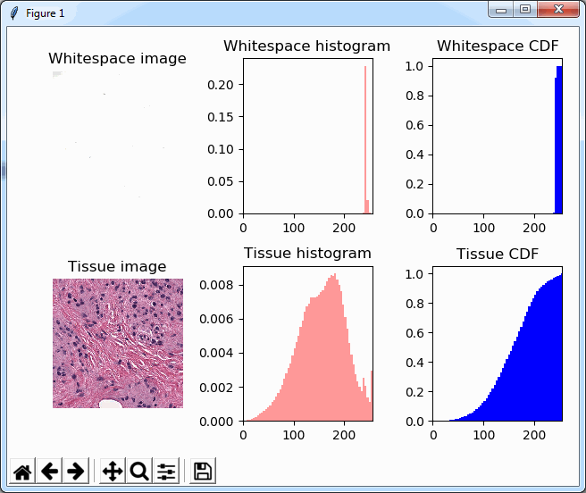
We can add a cumulative distribution function to further illustrate the difference:

# Display whitespace image
plt.subplot(2,3,1)
plt.title('Whitespace image')
plt.axis('off')
plt.imshow(tile_0_0, cmap="gray")

# Display a histogram of whitespace pixels
plt.subplot(2,3,2)
plt.xlim((0,255))
plt.title('Whitespace histogram')
plt.hist(pixels_0_0, bins=64, range=(0,256), color="red", alpha=0.4, normed=True)

# Display a cumulative histogram of the whitespace
plt.subplot(2,3,3)
plt.hist(pixels_0_0, bins=64, range=(0,256), normed=True, cumulative=True, color='blue')
plt.xlim((0,255))
plt.grid('off')
plt.title('Whitespace CDF')

# Display tissue image
plt.subplot(2,3,4)
plt.title('Tissue image')
plt.axis('off')
plt.imshow(tile_x_y, cmap="gray")

# Display a histogram of whitespace pixels
plt.subplot(2,3,5)
plt.xlim((0,255))
plt.title('Tissue histogram')
plt.hist(pixels_x_y, bins=64, range=(0,256), color="red", alpha=0.4, normed=True)

# Display a cumulative histogram of the tissue
plt.subplot(2,3,6)
plt.hist(pixels_x_y, bins=64, range=(0,256), normed=True, cumulative=True, color='blue')
plt.xlim((0,255))
plt.grid('off')
plt.title('Tissue CDF')

Note that we’re now using a 2 x 3 grid to display the histogram and the cumulative distribution function (CDF) next to each other, which ends up looking like this:

Back to basic (statistics)

We could now write a complicated method that manually scans through the pixel-arrays and assesses how many bins there are, how they are distributed etc. However, it is worth noting that the histogram-buckets that are NOT showing any values in the histogram, are not pixels-values of 0; the histogram shows a frequency, therefore, empty spaces in the histogram simply means that NO pixels are available at a given intensity.

So after we visualized the pixel distribution through MatPlotLib’s PyPlot, it’s worth looking as some basic statistics for the flattened pixels arrays. Numpy’s basic .std() and .mean() functions are good enough to do the job for now. The script becomes:

from pma_python import core
import matplotlib.pyplot as plt
import numpy as np
import scipy.stats

slide = "C:/my_slides/CMU-1.svs"
max_zl = core.get_max_zoomlevel(slide)
dims = core.get_zoomlevels_dict(slide)[max_zl]

# obtain whitespace tile
tile_0_0 = core.get_tile(slide, x=0, y=0, zoomlevel=max_zl)
# Flatten the whitespace into 1 dimension: pixels
pixels_0_0 = np.array(tile_0_0).flatten()
# print whitespace statistics
print("Whitespace Mean = ", np.mean(pixels_0_0))
print("Whitespace Std  = ", np.std(pixels_0_0))
print("Whitespace kurtosis = ", scipy.stats.kurtosis(pixels_0_0))
print("Whitespace skewness = ", scipy.stats.skew(pixels_0_0))

# obtain tissue tile
tile_x_y = core.get_tile(slide, x=int(dims[0] / 4), y=int(dims[1] / 2), zoomlevel=max_zl)
# Flatten the tissue into 1 dimension: pixels
pixels_x_y = np.array(tile_x_y).flatten()
# print tissue statistics
print("Tissue Mean = ", np.mean(pixels_x_y))
print("Tissue Std. = ", np.std(pixels_x_y))
print("Tissue kurtosis = ", scipy.stats.kurtosis(pixels_x_y))
print("Tissue skewness = ", scipy.stats.skew(pixels_x_y))

The output (for the same tiles as we visualized using PyPlot earlier is as follows:

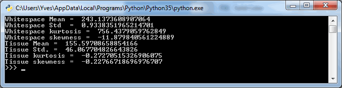
The numbers suggest that the mean-(grayscale-)value of a Whitespace tile is a lot higher than that of a tissue tile. More importantly: the standard deviation (variance squared) could be an even more important indicator. Naturally we would expect the standard deviation of (homogenous) whitespace to be much less than that of tissue pictures containing a range of different features.

Kurtosis and skewness are harder to interpret and place, but let’s keep them in there for our further investigation below.

Another histogram

We started this post by analyzing an individual tile’s grayscale histogram. We now summarized that same histogram in a limited number of statistical measurements. In order to determine whether those statistical calculations are an accurate substitute for a visual inspection, we compute those parameters for each tile at a zoomlevel, and then plot those data as a heatmap.

The script for this is as follows. Depending on your fast your machine is, you can play w/ the zoomlevel parameter at the top of the script, or set it to the maximum zoomlevel (at which point you’ll be evaluating every pixel in the slide.

from pma_python import core
import matplotlib.pyplot as plt
import numpy as np
import scipy.stats
import sys

slide = "C:/my_slides/CMU-1.svs"
max_zl = 6 # or set to core.get_max_zoomlevel(slide)
dims = core.get_zoomlevels_dict(slide)[max_zl]

means = []
stds = []
kurts = []
skews = []

for x in range(0, dims[0]):
    for y in range(0, dims[1]):
        tile = core.get_tile(slide, x=x, y=y, zoomlevel=max_zl)
        pixels = np.array(tile).flatten()
        means.append(np.mean(pixels))
        stds.append(np.std(pixels))
        kurts.append(scipy.stats.kurtosis(pixels))
        skews.append(scipy.stats.skew(pixels))
    print(".", end="")
    sys.stdout.flush()
print()

means_hm = np.array(means).reshape(dims[0],dims[1])
stds_hm = np.array(stds).reshape(dims[0],dims[1])
kurts_hm = np.array(kurts).reshape(dims[0],dims[1])
skews_hm = np.array(skews).reshape(dims[0],dims[1])

plt.subplot(2,4,1)
plt.title('Mean histogram')
plt.hist(means, bins=100, color="red", normed=True)
plt.subplot(2,4,5)
plt.title('Mean heatmap')
plt.pcolor(means_hm)

plt.subplot(2,4,2)
plt.title('Std histogram')
plt.hist(stds, bins=100, color="red", normed=True)
plt.subplot(2,4,6)
plt.title("Std heatmap")
plt.pcolor(stds_hm)

plt.subplot(2,4,3)
plt.title('Kurtosis histogram')
plt.hist(kurts, bins=100, color="red", normed=True)
plt.subplot(2,4,7)
plt.title("Kurtosis heatmap")
plt.pcolor(kurts_hm)

plt.subplot(2,4,4)
plt.title('Skewness histogram')
plt.hist(skews, bins=100, color="red", normed=True)
plt.subplot(2,4,8)
plt.title("Skewness heatmap")
plt.pcolor(skews_hm)

plt.tight_layout()
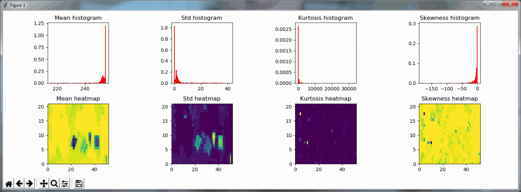
plt.show()

The result is a 2 row x 4 columns PyPlot grid, shown below for a selected zoomlevel of 6:

The standard deviation as well as the mean grayscale value of a tile seem accurate indicators to determine the position of where tissue can be found on the slide; skewness and kurtosis not so much.

Both the mean histogram and the standard deviation histogram show a bimodal distribution, and we can confirm their behavior by looking at other slides. It even works on slides that are only lightly stained (we will return to these at a later post and see how we can make the detection better in these:

A binary map

We can now write a function that determines whether a tile is (mostly) tissue, based on the mean and standard deviation of the grayscale pixel values, like this:

def is_tissue(tile):
    pixels = np.array(tile).flatten()
    mean_threahold = np.mean(pixels) < 192   # 75th percentile
    std_threshold = np.std(pixels) < 75
    return mean_threahold == True and std_threshold == True

Writing a similar function that determines whether a tile is (mostly) whitespace, is possible, too, of course:

def is_whitespace(tile):
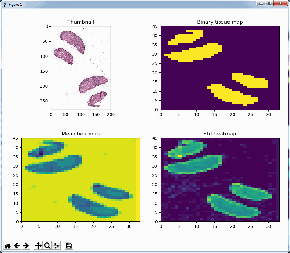
    return not is_tissue(tile)

Similarly, we can even use this function to now construct a black and white map of where the tissue is located on a slide. The default color map of PyPlot on our system nevertheless rendered the map blue and yellow:

In closing

This post started with “Let’s say that you have a great algorithms to distinguish between PDL1- and a CD8-stained cells.”. We didn’t quite solve that challenge yet. But we did show you some important initial steps you’ll have to take to get to that part eventually.

In the next couple of blogs we want to elaborate on the topic of tissue detection some more. We want to discuss different types of input material, as well as see if we can use a machine learning classifier to replace the deterministic mapping procedure developed here.

But first, we’ll get back to testing, and we’ll tell you why it was important to have the is_tissue() function from the last paragraph developed first.