Blurred or focused?
In an earlier post, we offered some ideas on how to detect tissue in a scanned slide.
The next step people often want to take is to examine how the sharpness of the tissue is distributed throughout the slide. No scanner catches all, and you will see blurry areas in pretty much all your scans.
It then helps to be able to differentiate the tiles that have poor focus from the tiles that are sharp. As it turns out, we already approached a likewise problem when we were determining the sharpest tiles within z-stacked slides.
For this particular exercise (focus variation within a single plane) Sied Kebir in Germany was kind enough to provide us with relevant sample data for this one.
And here are two relevant extracted tiles to illustrate the problem.
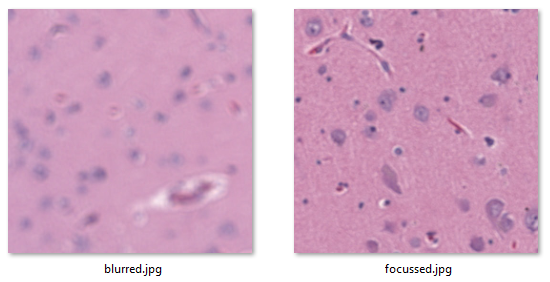
Sied is looking for a method to systematically map the blurry tiles vs the crisp ones.
Blur detection with OpenCV
A good introduction on blur detection with the OpenCV library is offered by pysource in the following video tutorial:
Let’s see what that gives when we apply it to Sied’s sample images:
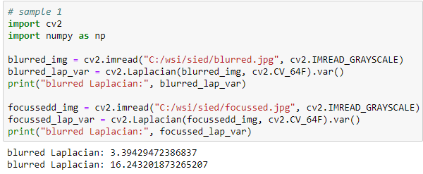
Great! The numbers are not as far apart as in pysource’s video, but that makes sense: even in focused tissue we’ll find many more gradients and sloping color ranges than in the average picture of person sitting a room, which contains distinctive features like outlined walls and facial contours.
Pysource suggests converting your original images to grayscale. Does it make a difference? In our experiments we find different values (of course), but the trend is the same. Since the retention color of leads to slightly bigger differences, we’re inclined to sticking with the original color images.
If you do want to convert your color tiles to grayscale, here’s a great StackOverflow article about how this works.
Distribution and Exploratory Data Analysis (EDA)
Our next step is to put it all in a loop and systematically examine how sharp or blurry each individual tile actually is. For semantic ease, we create a get_blurriness function:
from pma_python import core
import matplotlib.pyplot as plt
import numpy as np
import scipy.stats
import sys

def is_tissue(tile):
    pixels = np.array(tile).flatten()
    mean_threahold = np.mean(pixels) < 192   # 75th percentile
    std_threshold = np.std(pixels) < 75
    return mean_threahold == True and std_threshold == True

def is_whitespace(tile):
    return not is_tissue(tile)

def get_sharpness(img):
    pixels = np.array(img).flatten()
    return cv2.Laplacian(pixels, cv2.CV_64F).var()

slide = "C:/wsi/sied/test.svs"
max_zl = 5 # or set to core.get_max_zoomlevel(slide)
dims = core.get_zoomlevels_dict(slide)[max_zl]

means = []
stds = []
tissue_map = []
sharp_map = []

for x in range(0, dims[0]):
    for y in range(0, dims[1]):
        tile = core.get_tile(slide, x=x, y=y, zoomlevel=max_zl)
        tiss = is_tissue(tile)
        tissue_map.append(tiss)
        if (tiss):
            sharp_map.append(get_sharpness(tile))
        else:
            sharp_map.append(0)
    print(".", end="")
    sys.stdout.flush()
print()
After getting all the result, it is worth examining the histogram of this data.
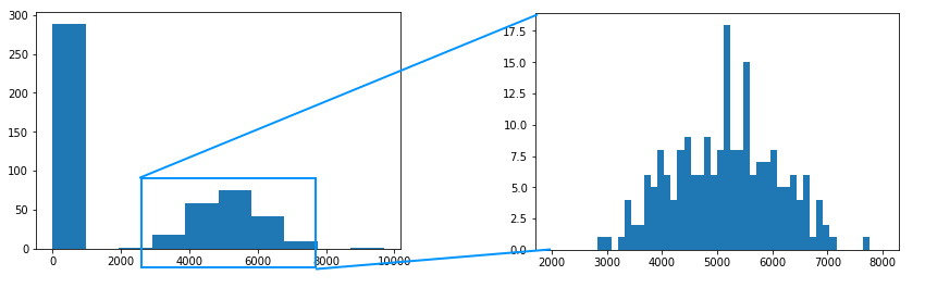
Ideally, we would like to see a bimodal distribution (sharp vs blurred), but that’s not what we see here. The reason is that unevenness in tissue is actually not distributed unevenly.
Putting it all together
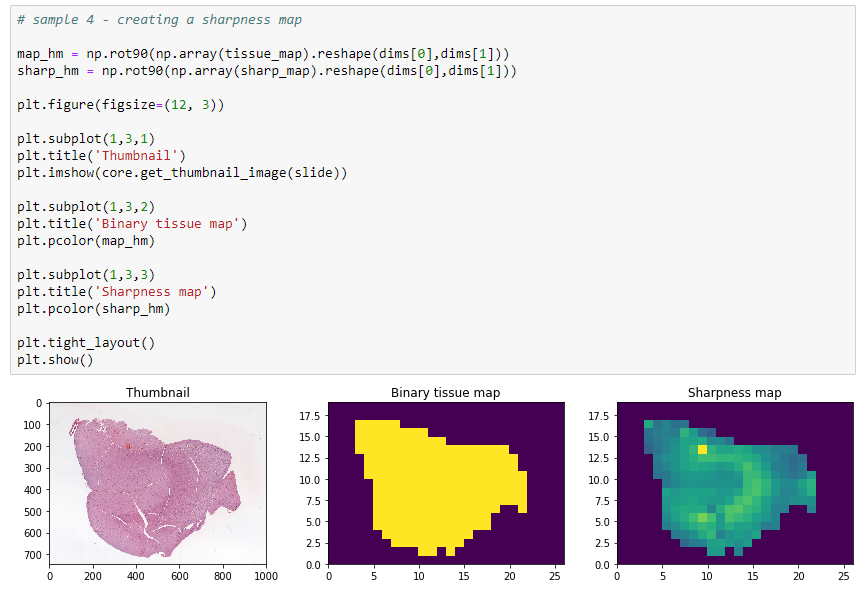
Now that we know what we can expect, it’s just a matter of putting it all together. and use it to construct an image map, in similar fashion as we did for our original tissue detection.
The final result looks like this:
In closing
Sectioning a slide is a continuous operation, and except for folding artifacts, you shouldn’t expect any abrupt changes. Tissue can be expected to gradually fade in and out of focus. And while scanners have gotten better at compensating for uneven tissue thickness, we’re not quite there yet, and automated analysis based on a technique like we’re here proposing can help.
Last but now least, we decided on a new way to organize our sample code. At http://host.pathomation.com/realdata/ you can from now on see all sample data in a single location. For example, the Jupyter notebook that belongs with this entry, is available at http://host.pathomation.com/realdata/jupyter/realdata%20033%20-%20look%20sharp.ipynb