We want talk a bit more about our different communication channels this week.
When you’re reading this article, you’ve obviously found one
of them.
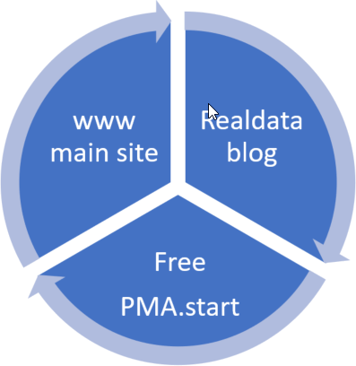
The RealData blog at http://realdata.pathomation.com is a
wordpress website that we set up a couple of years ago to allow us to
communicate about or explain topics that don’t necessarily have a dedicated
place yet on our “main” company website at http://www.pathomation.com.
Pathomation is a small company, and things can move quickly. We simply don’t have time to re-do our website each month or so because our product offering changes, or because there’s a spurt in creative writing that needs to find a landing spot and reach an audience. A free-form blog then seemed like a good idea.
And we still think it is 😊
There are companies whose website is a blog, but we
do think there’s still a need to offer structured information and a general
product overview as well.
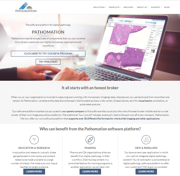
So while you can’t constantly rewrite your website, we did manage to re-work http://www.pathomation.com this month and we’re pretty proud of the result. If you haven’t checked it out yet, go ahead and do so. It’s a lot more comprehensive than anything we’ve had up before.
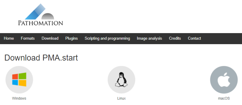
And if you’ve read this blog, of course you’ve heard about PMA.start before, our free whole slide image / digital pathology viewer software that can be used by anybody for anything to manage their local slide content. Our http://free.pathomation.com website is the third axis of our online web-presence strategy.
PMA.start comes with no limitations, except the one that is built-in: you can only use it on local content. If you want to share data with colleagues via a network, you need to upgrade to our professional PMA.core product. If you’re not quite sure what that’s all about, you can still sign up for our beta program until the end of this month (just a few days left, so be quick).
And there you have it; our three pronged strategy to provide you, our valued customer and end-user, with background information about the Pathomation universe, and our great products.
Pathomation’s software platform includes software for a number of digital pathology application.
At the most basic end of the spectrum we offer PMA.start for local viewing and research purposes. Even with PMA.start, you get full access to our front-end Javascript-based visualization framework, and back-end automation API (more on those in a separate blogpost).
At the opposite end of the spectrum, we offer a sophisticated training software package called PMA.control. Consider this:
Current slide-based approaches to microscopy
teaching face the logistical challenge of transporting people, slides and
training material.
The size, location and number of instructional sessions
is limited (in time, place, and size)
Concurrent training on the same material is not
possible. One microscope can offer one unique slide. Musical chair… erh…
microscopes, anyone?
We identified a need has evolved to train students and
professionals alike to accurately evaluate tissue material with a broad range
of (assay-specific) algorithms. Systematically organizing training materials and
bringing training participants together in a virtual settings, is what it’s all
about.
Projects
You start in PMA.control by setting up a project. A project describes what it is that you want to organize instructional material around. A project can represent a course at a university, or a drug for a pharma company. A project can delineate a geographical territory. It’s totally up to you.
Projects have various properties. Apart from their name, you can identify them with an icon. This is convenient as your list of project becomes larger and more people become involved in your project. Speaking of involved people: you can identify one or more project managers. This is particularly useful for larger organizations, where one person is seldom available all the time, but it’s relatively easy to find a replacement in case of absence.
Training sessions
A project consists of training sessions. Again, what these mean
semantically is completely up to you and your imagination:
One client of ours uses PMA.control to organize
weekly seminars in various places across the globe. Each seminar/country
combination translates into its own training session in PMA.control, with
specific start- and end-dates
One medical school uses PMA.control to train
residents. A training session can refer to the class coming in on a particular
week, but it can also be linked to small research projects that students
participate in.
Another client integrates PMA.control into a
web-portal, so all training sessions by definitions are open ended. The client
has a drug portfolio, so rather than have them be restricted in time, training sessions
refer to various indications for different drugs.
Safe to say that training sessions can be exploited for diverse applications.
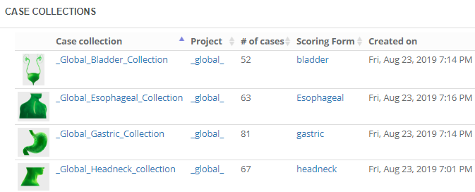
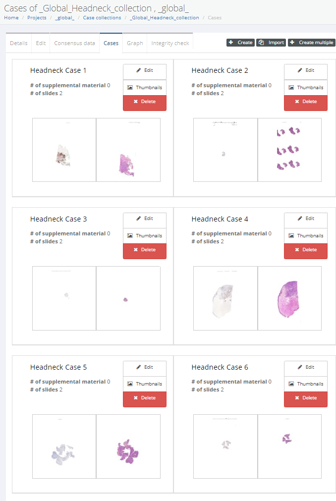
Case collections
All right, we have projects and training sessions… When do we
put digital slide content in them? This is where case collections come in.
The idea is that you organize your training sessions in
different parts. During a three-day seminar, you could have one day dedicated
to guided lectures (that’s a case collection with its own slides). On day two,
you allow people to evaluate themselves through some hands-on exercises (on a
second case collection, which holds different slides than the first one). On
day three, it’s crunch time, and attendees take an actual test to see how well
they absorbed the material (on yet another third case collection with once again
unique slides).
A case collection is coupled to a project, but is independent from any training sessions, so you can re-use them throughout the curriculum that you’re building. Think about it; otherwise if you organized the same training session repeatedly, you would continuously have to re-define the case collections, too!
A case collection consists of cases, which in turn consist of slides. You can choose to construct a case such that it pre-focuses on a particular region of interest (ROI) within a slide. You can also add various meta-data at case-level as well as slide-level. Not unimportantly: you can configure the initial rotation angle for each slide in the case. This is particularly relevant if your case consists of serial sections that may not be all in the exact same orientation.
Interaction modes
Remember the three-day seminar we just mentioned? And you
also remember that we called the software “PMA.control”, right?
Ok.
The name PMA.control refers to the fact that the owner of
the software is in total control of what participants within a session at any
given time.
Consider the following situations during our three-day seminar:
On the first day, the instructor wants his pupils
to stay nicely in the kiddie pool. They should give their undivided attention only
to the material intended for the first day.
However, this one person in the afternoon of the
first day is taking the seminar for the second time. She asks if she can skip ahead
already to the content from day two.
On the second day, people are learning and
experimenting with a different dataset. Do they understand the material well
enough to pass the test on the last day? Clearly the material from day three
must not be visible to anybody yet.
On day three, it’s crunch time. The actual test
material is now released. Depending on the intention of the instructor, earlier
discussed material can now even be closed off.
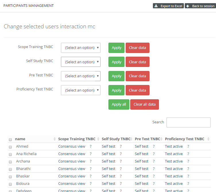
For all these conditions, PMA.control offers interaction
modes. An interaction mode controls if and how a case collection presents
itself to the end-user.
Training sessions consist of multiple case collections and
multiple users participate in a training session. At any given time, the
instructor of a session can specify whether a particular case collection within
the session is accessible to a specific user and how.
When signing into PMA.control, the instructor sees a grid with users and case collections. This grid can be used to control what user interacts with what case collection.
PMA.control ships with a number of default interaction modes, but these can be customized via a matrix interface where one stipulates what properties are associated with each.
Let’s see how interaction modes come into play during our
three-day seminar:
Before leaving for the seminar, the instructor applies the interaction mode “locked” to all case collections for all participants.
On the morning of the first day, the instructor walks in the seminar room an hour early an sets the interaction mode of the first case collection to “browse” for everybody to see. That was easy! He goes to the hotel bar to grab a nice cup of coffee.
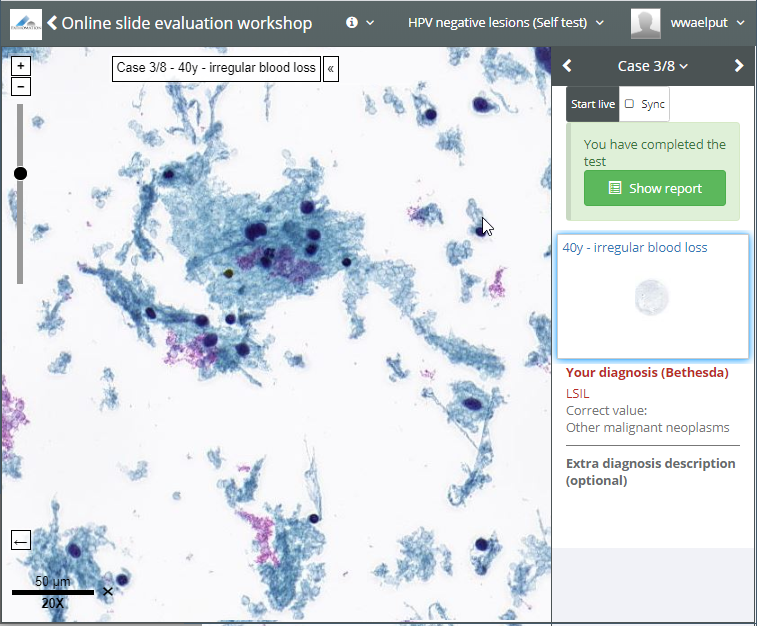
In the afternoon of the first day, an attendee asks about being allowed to skip ahead with the material a bit. The instructor asks if any other people are in the same situation. For those, he sets the interaction mode for the second case collection to “self-test”. Users can interactively fill out a pre-determined scoring form that goes with each case, and they can see each other’s results to discuss their findings amongst themselves.
On the second day, the second case collection is unlocked for everybody. Everybody now sees the second case collection in self-test mode. The first case collection remains in “browse” mode, so participants can use these as reference material. The third case collection remains off limits today.
On the morning of the third day, the first thing the instructor does is reset the first and second case collection in the training session to “locked”. Rien ne va plus. The third and last case collection is switched to “test”, and students can take their final assessment. Users can interactively fill out a pre-determined scoring form that goes with each case, but they can’t see each other’s data anymore.
It’s possible for an instructor to be an instructor for one
session, but only a “regular” participant in another. This is especially useful
in medical schools where different specialists consult with and train each other
on various subject matters on a continuous basis.
Conclusion
PMA.control allows you to assemble whole-slide images, scoring forms, consensus scores and scoring manuals into digital training modules. Full service, no-hassle, management of the software is offered through the PathoTrainer service, which is organized through Pathomation’s parent company CellCarta .
In an earlier post, we offered some ideas on how to detect tissue in a scanned slide.
The next step people often want to take is to examine how the sharpness of the tissue is distributed throughout the slide. No scanner catches all, and you will see blurry areas in pretty much all your scans.
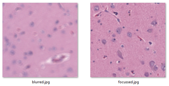
For this particular exercise (focus variation within a single plane) Sied Kebir in Germany was kind enough to provide us with relevant sample data for this one.
And here are two relevant extracted tiles to illustrate the problem.
Sied is looking for a method to systematically map the
blurry tiles vs the crisp ones.
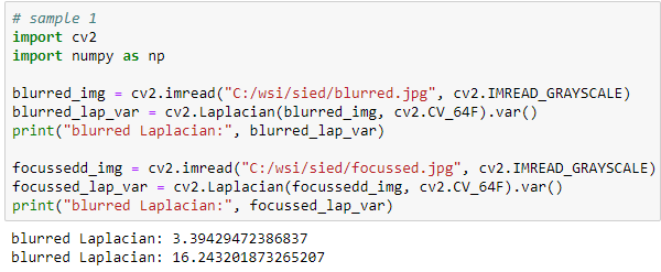
Blur detection with OpenCV
A good introduction on blur detection with the OpenCV library is offered by pysource in the following video tutorial:
Let’s see what that gives when we apply it to Sied’s sample images:
Great! The numbers are not as far apart as in pysource’s video, but that makes sense: even in focused tissue we’ll find many more gradients and sloping color ranges than in the average picture of person sitting a room, which contains distinctive features like outlined walls and facial contours.
Pysource suggests converting your original images to grayscale. Does it make a difference? In our experiments we find different values (of course), but the trend is the same. Since the retention color of leads to slightly bigger differences, we’re inclined to sticking with the original color images.
If you do want to convert your color tiles to grayscale, here’s a great StackOverflow article about how this works.
Distribution and Exploratory Data Analysis (EDA)
Our next step is to put it all in a loop and systematically examine how sharp or blurry each individual tile actually is. For semantic ease, we create a get_blurriness function:
from pma_python import core
import matplotlib.pyplot as plt
import numpy as np
import scipy.stats
import sys

def is_tissue(tile):
    pixels = np.array(tile).flatten()
    mean_threahold = np.mean(pixels) < 192   # 75th percentile
    std_threshold = np.std(pixels) < 75
    return mean_threahold == True and std_threshold == True

def is_whitespace(tile):
    return not is_tissue(tile)

def get_sharpness(img):
    pixels = np.array(img).flatten()
    return cv2.Laplacian(pixels, cv2.CV_64F).var()

slide = "C:/wsi/sied/test.svs"
max_zl = 5 # or set to core.get_max_zoomlevel(slide)
dims = core.get_zoomlevels_dict(slide)[max_zl]

means = []
stds = []
tissue_map = []
sharp_map = []

for x in range(0, dims[0]):
    for y in range(0, dims[1]):
        tile = core.get_tile(slide, x=x, y=y, zoomlevel=max_zl)
        tiss = is_tissue(tile)
        tissue_map.append(tiss)
        if (tiss):
            sharp_map.append(get_sharpness(tile))
        else:
            sharp_map.append(0)
    print(".", end="")
    sys.stdout.flush()
print()
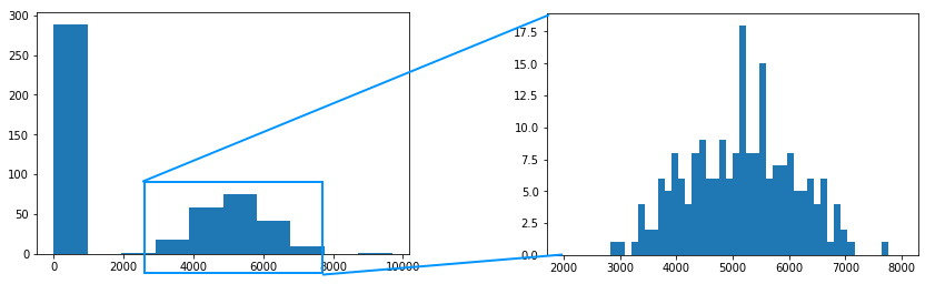
After getting all the result, it is worth examining the histogram of this data.
Ideally, we would like to see a bimodal distribution (sharp vs blurred), but that’s not what we see here. The reason is that unevenness in tissue is actually not distributed unevenly.
Putting it all together
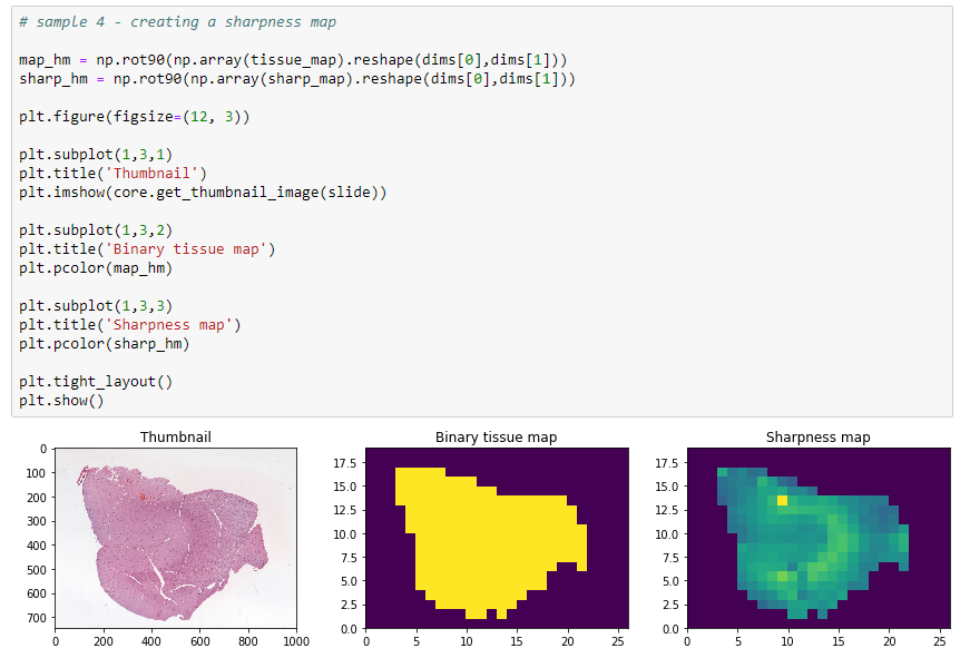
Now that we know what we can expect, it’s just a matter of putting it all together. and use it to construct an image map, in similar fashion as we did for our original tissue detection.
The final result looks like this:
In closing
Sectioning a slide is a continuous operation, and except for folding artifacts, you shouldn’t expect any abrupt changes. Tissue can be expected to gradually fade in and out of focus. And while scanners have gotten better at compensating for uneven tissue thickness, we’re not quite there yet, and automated analysis based on a technique like we’re here proposing can help.
This website uses cookies to improve your experience. We'll assume you're ok with this, but you can opt-out if you wish. Cookie settingsACCEPT
Privacy & Cookies Policy
Privacy Overview
This website uses cookies to improve your experience while you navigate through the website. Out of these cookies, the cookies that are categorized as necessary are stored on your browser as they are essential for the working of basic functionalities of the website. We also use third-party cookies that help us analyze and understand how you use this website. These cookies will be stored in your browser only with your consent. You also have the option to opt-out of these cookies. But opting out of some of these cookies may have an effect on your browsing experience.
Necessary cookies are absolutely essential for the website to function properly. This category only includes cookies that ensures basic functionalities and security features of the website. These cookies do not store any personal information.
Any cookies that may not be particularly necessary for the website to function and is used specifically to collect user personal data via analytics, ads, other embedded contents are termed as non-necessary cookies. It is mandatory to procure user consent prior to running these cookies on your website.