Pop quiz
Let’s start this post with a pop-quiz. Without peeking ahead; can you identify what painting it is?

The answer of course is that it’s this one. The question is relevant, because you just proved to yourself that you can get by with very little information to identify something big and important. So let’s just walk you through the way we created the picture above:
- We took the original image from Wikipedia, provided through the WikiMedia Commons library, at 585 x 870 pixels (a total of 508,950 pixels). The physical size of this image was 957 KB.
- We then resized this image to thumbnail size of 27 x 40 pixels (a total of 1,080 pixels, or a reduction by 99.8%). The physical size of this image was around 3 KB (a reduction by 99.7%).
- We then blew up the thumbnail again with a factor 10 to 270 x 400 pixels (bringing the total amount of pixels again to 108,000 or about 21% of the original). Interestingly enough, the image size this time is 75 KB, which represents only about 8% (even though we supposedly offer 21% of the original pixels).
The important takeaway is that the human brain is remarkable in filtering out and handling noisy, blurry data.
But what does this have to do with digital pathology or virtual microscopy?
A bottleneck
Recently we were contacted by a company that was involved in telepathology in rather rural areas. It’s a great endeavor: they provide local staff with refurbished scanners, thereby hoping to extend advanced pathology expertise to communities that have no other way of having access to these.
But as anybody working with whole slide images can attest: they’re big. Huge sometimes, And there’s no way around this. And it’s a problem for our contact because rural areas unfortunately oftentimes also still mean limited bandwidth. It can take hours to transfer a single slide, and that’s just not practical.
This is where our earlier exercise comes into play. And the question now becomes: How much information do you really need to make an accurate diagnosis?
If we scan a slide at 40X (0.25 ppm according to DICOM’s definition) and we brought it back down to 20X (0.5 ppm), would it be sufficient for a pathologist to make an accurate diagnosis? And what about image compression? Do we need 100%? What if we transferred the image with 90% quality? 80%? We know that at 50% compression artifacts will not result in a pretty image, but the real question is whether the receiving pathologist can still make a diagnosis.
Some research has done on this: Yukako et al concluded that even significant compression ratios have no impact on diagnostic accuracy.
So with that being said, how could you do it? And how would you do it with the Pathomation platform?
To Jupyter, capt’n!
A whole slide image has two properties that we can manipulate to control the physical slide size:
- The highest zoomlevel contained in the slide (see also our blog post of WSI structure)
- The compression ratio of individual tissue tiles
We can then create a jupyter script can takes in these two parameters, to convert any given slide to an intermediate format. We choose TIFF here, but you can adapt the output to your own needs.
The first one is target-quality, and can be given a value of 0-100 (100 being the highest quality).
The second one is the downscale factor. It can be chosen from a list of values of [1, 2, 4, 8, 16, 32, 64, 128]. That doesn’t quite translate to an optical magnification or pixels per micron reading, but we use it here for the sake of simplicity (it has to do with the way these WSI data are typically structured). The higher the downscale factor, the less magnification and detail you will end up with. If you want to, you can write your own conversion method from downscale-factor to ppm and back again.
After setting the parameters, we create new TIFF file using the GDAL TIFF driver. The width and height of the final tiff is based on number of tiles horizontally and vertically.
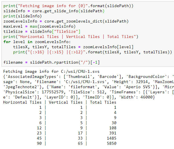
We read each tile of the final zoomlevel (1:1 resolution) from the server and write it to the resulting TIFF file Then we create the pyramid of the file using BuildOverviews function of GDAL
The complete Jupyter notebook is available from our website.
The jury is in session
Let’s see what the result of our code is for different combinations.
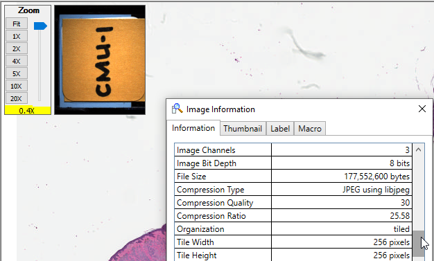
We downloaded CMU-1.svs from the OpenSlide sample data repository, which has a compression quality of 30%. The original file size is 169 MB.
When we run our script and ask to generate a derived TIFF slides with 100% tile quality and the same magnification level, we find something interesting: the new slide is about 1.5 GB is slide. It became bigger!
This is our first lesson then: when doing these kind of conversions, it doesn’t make any sense to transfer data at a compression rate that’s lower than the original slide’s compression.
The CMU-1.svs slide is an extreme case. We haven’t heard of any labs that are scanning at only 30% quality; most scanners are usually calibrated to produce data at 70%-80% compression quality.
That being said, let’s just use the 1.5 GB as a reference point and see how the data package becomes smaller as we vary both the compression quality and the downsampling parameter:
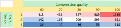
Not surprisingly, as the scaling factor goes up (a scaling factor of 4 would roughly correspond with a perceived magnification of 10X), the resulting slide size becomes significantly smaller.
So in both axes, significant saving are to be had. Similar to the Mona Lisa painting example that we started with; the slide at 10X and 60% quality is only 2.3% the filesize of the original 40X and 100% quality file.
What else?
We wrote this article to give you ideas on how you can employ PMA.start to optimize your data volume when shuttling back data back and forth between two sites.
This is but one scenario to consider. Is the eventual resolution sufficient to maintain diagnostic accuracy? That’s up to you and your pathologist(s) to resolve. Whether the parameters specified here work for you, is a question you can only answer.
To give you an idea; here’s the slide with a downsampling rate of 1, and 100% compression quality:
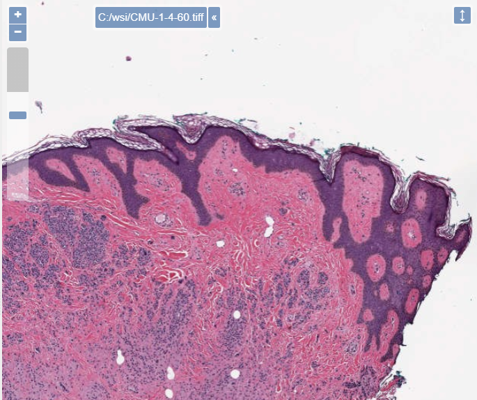
Here’s the same slide with a downsampling rate of 4, and only 60% compression quality:

There is one more interesting experiment to consider here: storage for digital pathology doesn’t scale very well, and we would be interested to see whether machine learning algorithms (ML/DL/AI) could be trained equally well on heavily compressed data, compared to uncompressed data.
Full disclosure here: There are things missing here, too. We’re not incorporating the thumbnail image in the exported TIFF, in similar fashion as certain other vendors do this. It’s possible, but again, the eventual implementation depends on your personal preference and circumstances. If you’re looking for help and advice with this, we can assist you and you may contact us at slides@pathomation.com.