A comprehensive look at image metadata
Whole Slide Images not only contain pyramidical giga-pixel images, but also various lower-resolution images with helpful information.
Image metadata
The type of image data that can be retrieved from an individual virtual slide is described at https://docs.pathomation.com/pma.core/3.0.2/doku.php?id=nonapi.
Three of these endpoints can be classified as image metadata:
- Thumbnail: A thumbnail image of the scanned slide. A low-resolution representation of the area of the glass slide that was scanned.
- Macro: A macro image of the entire slide (typically generated by a separate low-resolution camera that’s part of the slide scanner)
- Barcode: the label pasted on the slide. It’s possible for this paper label to contain a barcode. If this is the case, it is possible to interpret the barcode through a separate API call.
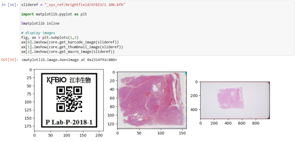
Here’s what all three images can look like for a particular slide:
The tile and region endpoints are related to selective pixel extraction and are irrelevant for the context of this article.
Macro images
The macro image shows the entire glass slide and offers an overview of all the tissue fragments present on the slide. A thumbnail represents the area of the slide scanned at high resolution. In case the tissue recognition of the scanner missed a tissue fragment, the tissue visible in the thumbnail will not match with the macro. Checking for mismatches in tissue between macros and thumbnails is an important quality control step in digital pathology.
But whole slide image are complex data structures. Not all file formats from all vendors therefore support all possible features and not all file formats from all vendors contain all metadata described here. This is obvious for the JPEG and PNG file formats.
Currently PMA.core supports macro images for twelve file formats:
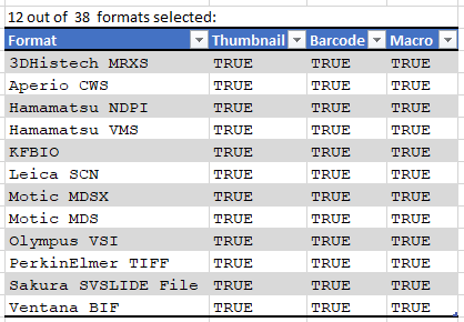
And here’s the code that we used to determine that output:
import pandas as pd
from pma_python import core

core.connect("http://server/pma.core/", "us3rn4m3", "S3CR3T!")

format_features = {}

def get_associated_image_types(slide):
    info = core.get_slide_info(slide)
    return info["AssociatedImageTypes"]

def get_file_format(slide):
    info = core.get_slide_info(slide)
    for item in info["MetaData"]:
        if (item["Name"].lower() == "fileformat"):
            return item["Value"]
    return ""

slides = core.get_slides("_sys_ref/brightfield", recursive = True)

for slide in slides:
    fmt = get_file_format(slide)
    if len(fmt) > 0:
        if not(fmt in format_features):
            format_features[fmt] = {"Thumbnail": False, "Barcode": False, "Macro": False}
        for tp in get_associated_image_types(slide):
            format_features[fmt][tp] = True

formats = pd.DataFrame.from_dict(format_features, orient="index")
macro_formats = formats[formats["Macro"] == True]

print(len(macro_formats), "out of ", len(formats), " formats selected:")
print(macro_formats)
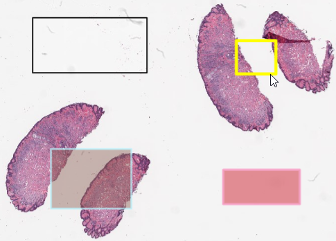
We can write PHP code that generates a catalog of all slide features in a single overview:
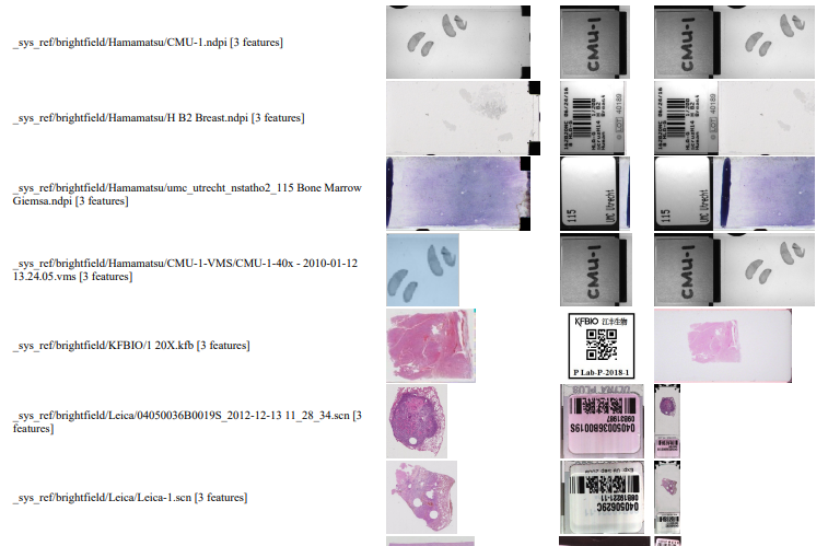
Note that the orientation of the macro-images can vary from one file format to the next: some opt for a vertical positioning, others for a vertical one. All of this can be compensated for, but it has repercussions: for example, if you rotate the macro images from Leica, it is useful for rotate the thumbnails the same way; otherwise comparison between macro and thumbnail becomes complicated.
Also note that with some vendors, the macro image is interpreted as “complete slide surface, including barcode”, whereas for others the macro image is the glass area of the slide, minus the label area.
The PHP source code reads like this:
<html>
<head><title>All meta features</title></head>
<body>
<?php
require_once "php/lib_pathomation.php";
Use  Pathomation\PmaPhp\Core;
$session = Core::connect("https://server/pma.core/", "us3rn4m3", "S3CR3T");
// echo "PMA.core SessionID = ".$session."<br>";
?>
<table>
	<tr><th>Format</th><th>Barcode</th><th>Thumbnail</th><th>Macro</th></tr>
<?php
$slides = Core::getSlides("_sys_ref/brightfield", $session, true

foreach ($slides as $slide) {
	$info = Core::getSlideInfo($slide, $session);
	$fc = count($info["AssociatedImageTypes"]);
	if ($fc > 2) {
		echo "<tr>
			<td>$slide [".$fc." features]</td>
			<td><img src='".Core::getBarcodeUrl($slide, $session)."' height=100></td>
			<td><img src='".Core::getThumbnailUrl($slide, $session)."' height=100></td>
			<td><img src='".Core::getMacroUrl($slide, $session)."' height=100></td>
			</tr>";
	}
}
?>
</table>

</body>
</html>
Image encoding hack (how to generate comprehensive reports)
You could use the above script as a starting point to generate daily overview reports of what’s been scanned. The output is “just” HTML in a browser, but comes with a disclaimer: Depending on the method used to convert the live page into an actual static report, may loose the images in the process.
A way around this is to switch from URL reference to base64 image encoding; like this:
function includeThumbnail($slide, $session) {
    $img = Core::getThumbnailImage($slide, $session);
    $img_data = base64_encode($img);
    return "data:image/jpg;base64,".$img_data;
}
The result of using this code is that the HTML file is now a single self-contained document. You can use it as an attachment, or share it through instant messaging (IM), without the need for anybody to have access to underlying image files or access to the original PMA.core tile server.
Interactive demo
We have an interactive demo available, too. This one was built with the JavaScript PMA.UI framework:
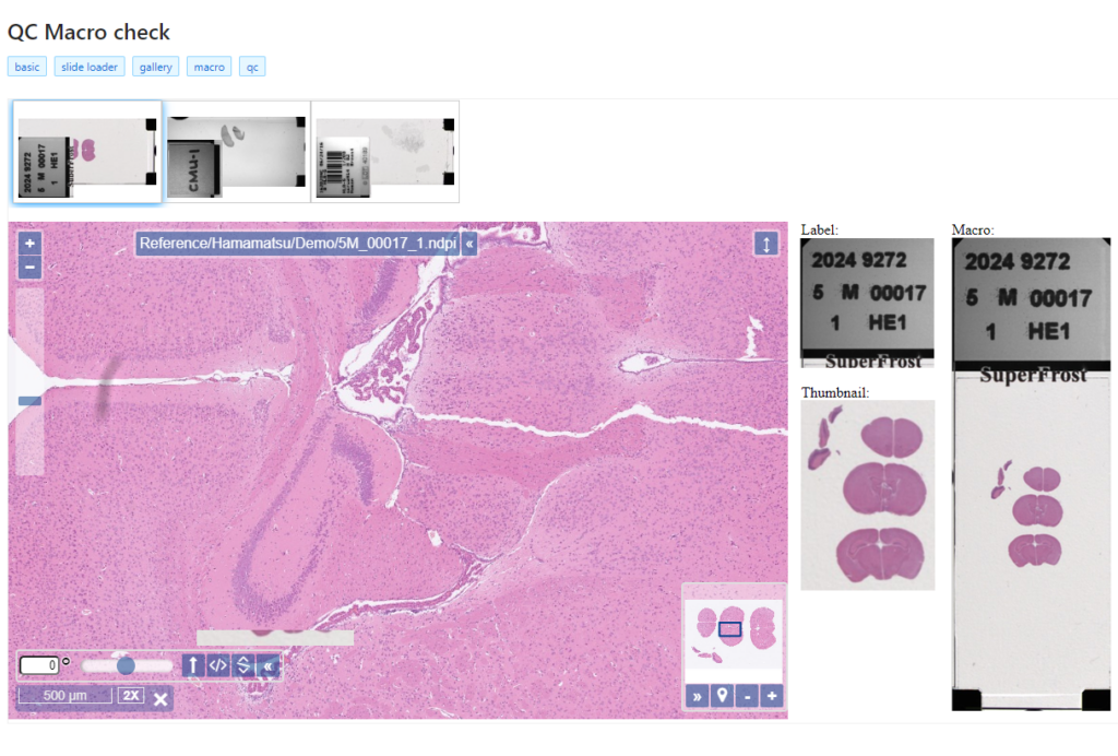
The demo is available through our JavaScript demo portal. We offer it as an inspiration as to what a custom QC module could look like.
In terms of workflow automation, you could write an algorithm that does tissue detection on both the thumbnail image, as well as the macro image, and compares the results. If the result is too divergent (or if the area of detected tissue falls below a pre-determined threshold), you could flag the slides as possibly faulty and send them to a lab technician for closer inspection.
Platform meta-data
Our SDKs are designed in such a way that they encapsulate typical plumbing code that would otherwise be needed to invoke the API-calls directly. When we do our job right, your Python script shouldn’t need the requests library anymore; your Java application shouldn’t need the java.net namespace anymore.
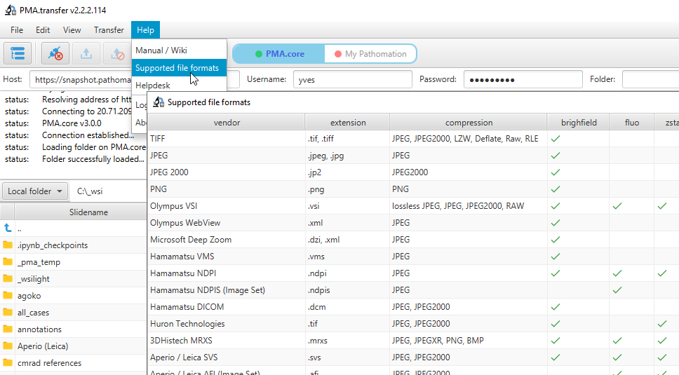
But our Pathomation platform itself has meta-data, too: like the file formats it supports.
When you’re an OEM solution provider that’s relying on our SDK to incorporate digital pathology features in your own software, you may want to offer a way for your own customers to see what file formats you support (through PMA.core then).
Therefore, we recently added a new call so people can programmatically request what modalities of what file formats we support. You get a JSON structure back, and you can render it to your own liking, which results in a nicer and smoother user experience on your end. We’re using this ourselves in PMA.transfer (as an alternative to opening a new webbrowser and pointing to https://www.pathomation.com/formats):
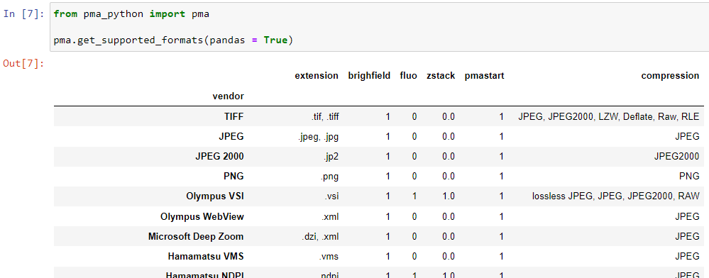
In Python, you can even choose whether to return results as a list, or as a pandas DataFrame object:
Platform meta-data
A picture says more than a thousand words, but is worth nothing without being placed in the right context. Without meta-data, those WSI virtual slides stored as gigapixel images are just that: pixels. Pathomation’s software platform for digital pathology (and the PMA.core tile server specifically) offers various opportunities to switch back and forth between (visual) slide metadata and pixels.
This is how Pathomation allows its customers to implement optimal workflows for digital pathology. Interested to switching over to Pathomation so you can exploit this kind of fine-grained granularity and customization too? Contact us today to discuss migration possibilities.
Four ways to add annotations to PMA.core (using Python)
PMA.core is a tile server that supports the creation of annotations on top of whole slide images.
The annotations are stored in the PMA.core back-end database as WKT strings. In the past, we’ve written about the different kinds of WKT strings that can be used to encode diffirent shapes of annotations, as well as what format is best suited to scale for greater volumes of annotations.
In this article we show the different ways the PMA.python SDK allows for the creation of annotations programmatically.
Random WKT rectangles with Python
Since this article is about how to define annotations in PMA.core, we decided to keep things simple and work with simple rectangles.
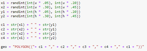
A rectangle in WKT is defined by 5 (x, y) coordinates: 4 corners, with a fifth point that traces back to the original corner to close the POLYGON loop.
We start by generating four x and y coordinates x1, x2, y1, y2 that will define the boundaries of the rectangle. We then use these to define (x, y) tuples, and combine them in a WKT string:
If you want to create more complex annotations, you can of course. the geo variable can contain any WKT-compatible annotation. And if you really want to go all out, have a look at the Python Shapely library as well, which contains a wrapper around the WKT syntax.
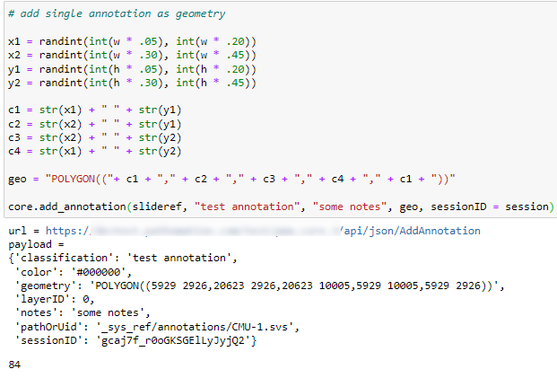
Storing single annotations
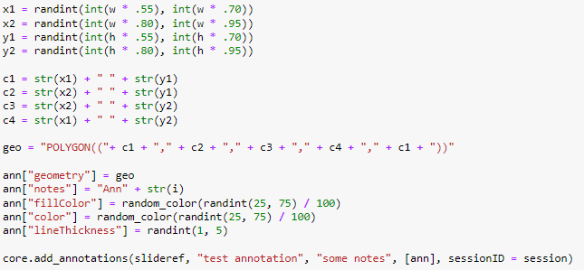
Once we have the WKT string, the most direct way to save the annotation is to pass it along with the add_annotation() call, like this:
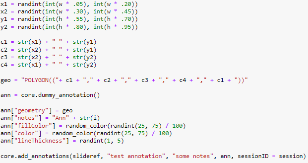
As people have started using our SDK more frequently, we’ve also been asked for additional features. Just so we wouldn’t have to keep adding parameters to the add_annotation() call, we now also offer the option to pass a dictionary along instead of a single WKT geometry string. For convenience, we offer a separate method that returns a blank dictionary with the appropriate keys filled out already (you determine the appropriate values):
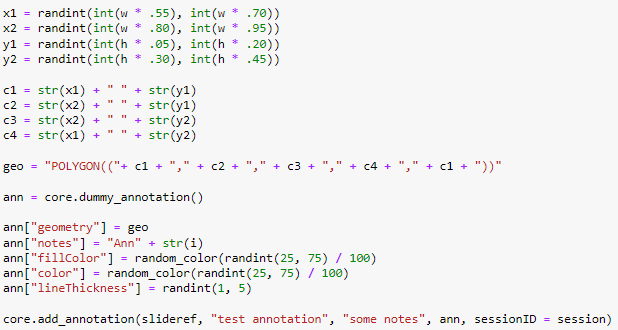
As you can see we can provide much richer styling of our annotation, without changing the syntax of the add_annotation() call; we simply pass the dictionary along, rather than the WKT geometry-string (which becomes part of the dictionary itself).
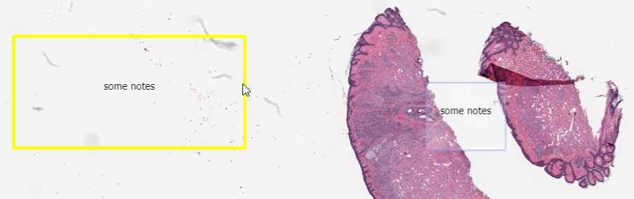
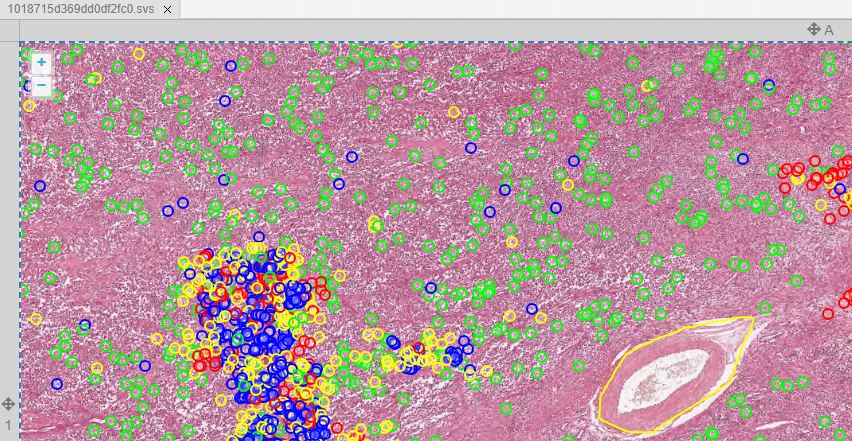
After running these two snippets of code, we end up with two random rectangles; one in the top-left, and another one in the top-right quadrant of our slide.
One, many, lots!
In our previous article we talked about performance matters, and how the right formatting and grouping of your WKT strings matter just as much.
When you have a lot a annotations to pass along, it’s faster to pass them along in a single call as an array, rather than having to invoke the same method over and over again.
This is why in addition to add_annotation(), there’s a new call introduced as of PMA.python revision 171 that allows for an array to be passed along instead of a single annotation.
Let’s look at the trivial example of passing along an array with just one element:
If you want to do a gradual conversion of your code from one type of interface to the next, you can also just replace your add_annotation() with add_annotations() calls. The latter is smart enough to figure out whether the passed argument is a list or not; if it’s not a list, the code will automatically adapt. The following lines of code are therefore equivalent:
core.add_annotations(slideref, "class", "notes", ann, sessionID = session)core.add_annotation(slideref, "class", "notes", ann, sessionID = session)The full code to fill up the fourth quadrant on our sample slide becomes like this:
Now it’s your turn!
The sample code from this article is available as a Jupyter notebook from our website.
How to handle hundreds of thousands of annotations?
In our latest article we discussed how Pathomation works with large enterprises and OEM vendors to continuously improve its SDK facilities and specific programming language support.
Once customers are satisfied with our interfaces, the next question usually is about scaling: they figured out how to programmatically convert a JSON file from an AI provider into WKT-formatted PMA.core annotations, but what if there are hundreds, thousands, or even hundreds of thousands of spots to identify on a slide?
First scalability checks
How do you even define scalability? Yes, everything must always be able to handle more stuff in less time. That’s rather vague…
Visiting conferences helped us in this regard: looking around, we discovered sample data sets that others were using for validation and stress testing. One such dataset is published through a Nature paper on cell segmentation. We also refer to this dataset in our Annotations et al article.
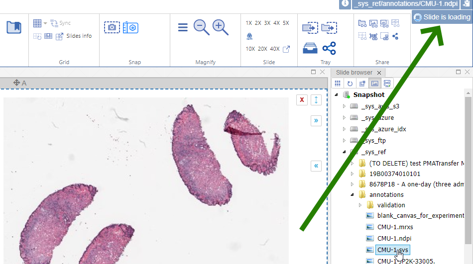
We obtained the code from https://github.com/DeepPathology/MITOS_WSI_CCMCT and got to work, scripting the conversion from the native (SQLite) format to records in our own (Microsoft SQLServer) database. 750,000 records were processed this way. A snapshot of just one slide is shown below in PMA.studio:
We admit we cheated to do the original import: Back in 2016, we didn’t have all the necessary and flexible API calls in PMA.core yet, let alone the convenient SDK interfaces for Python, PHP, and Java. So we used a custom script that translated the native records from the Nature paper into direct SQL statements. Not for the faint of heart, and only possible because we understand our own database structure in detail.
This initial experiment dates back a few years ago already (2016!). Today, you would solve this kind of problem through an ELT or ETL pipeline in an environment like Microsoft Azure Data Factory.
A more systematic approach
Fast-forward to last year. In 2022, we published a series of articles on software validation. Initial user acceptance testing – UAT – focuses on functionality however rather than scalability.
Can we exploit this mechanism to examine scalability as well? Or at least keep an eye on performance?
The way our approach works: we write out a User Requirement Specification – URS – that then gets its own UAT. The UAT is a Python Jupyter Notebook (using PMA.python) script. This script consists of different blocks that can be executed independently of each other.
The different kinds of annotations and how these translate to WKT-strings (as stored in our database) is described in a recent article on PMA.studio. The corollary for testing means that each cell in the Jupyter Notebook can test one specific type of annotation.
Linear scaling
Our first extension involved writing loops around our already in place test-code for the various types of annotations. The question we’re effectively asking: if it takes x amount of time to store a single annotation of type y; does it take n * x amounts of time to store n annotations?
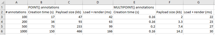
The test results below suggest it does:
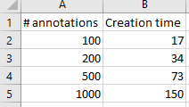
We were really excited with the results achieved. Our data shows that creating new annotations is a linear process: registering 1000 annotations takes roughly 10 times longer than registering 100 annotations. Inserting the 1000th annotation takes the same amount of time as inserting the 1st, 100th, 200th, or 500th annotation.
Loading and rendering considerations
Storing and retrieving data are different operations.
Our original data shows the times needed to create annotations. Luckily, it doesn’t take nowhere nearly as long to load and render annotations. But it still has some impact: more annotations will impact loading (and rendering) times in environments like PMA.studio. Below are the payload sizes and loading times of the same annotations we just created:
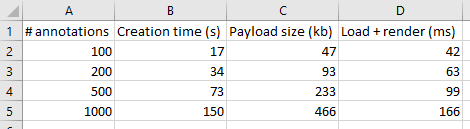
The conclusion from the table is that while 1000 annotations take 10 times longer to generate, and are 10 times larger in payload, they only take 4 times longer to load and render. That’s good!
But at the same time there is clearly a (albeit explainable) performance degradation as the annotation payload for a slide increases.
This is where user feedback becomes important, as well as (user) expectation management. A “slide loading” event can result in visual feedback like a spinning wheel cursor. In PMA.studio this is tackled by a status update in the top-right corner of the interface.
Keep in mind that the tests described here are performed in Jupyter notebooks. When we open one of the mitosis slides with real-world annotations, we find that it takes 9 seconds to load an annotation payload of 6.1 MB. The slide in question contains 13,781 annotations.
A better mousetrap for many landmark annotations
Our examples in the paragraph above indicate that we’re going to get into trouble with real-world datasets. We estimate that when, doing whole slide image analysis for something as mundane as a Ki67 marker (e.g. through interfacing with an external AI provider), we end up with anywhere between 100,000 and 200,000 individual cells, and therefore landmark annotations in PMA.core and PMA.studio. Extrapolating our earlier findings; it would take over 40 seconds to load these (and a payload of 4 MB)!
A MULTIPOINT annotation provides an alternative over individual POINT annotations then. Think of a multipoint annotation as a polygon, but without the lines. You can also think of these as a disconnected graph with only vertices and no edges.
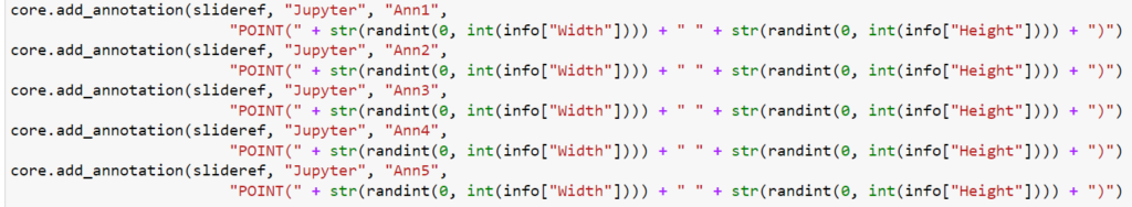
Let’s start with a simple example: let’s create 5 landmark annotations on a slide, by placing individual POINT annotations on them:
Let’s do the same via a MULTIPOINT annotation:
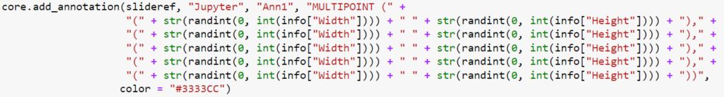
Even if you don’t read Python code, you can still see that the POINT annotations require the creation of five (5) annotations, whereas the MULTIPOINT annotation only requires one. Consequently, the first code snippet takes 0.71 seconds to execute; the second one only 0.14.
MULTIPOINT annotations are therefore the preferred way to go when you have a lot of individual cells to annotate. This is how the results compare to our original tests:
You can get more technical (WKT syntax) related information on MULTIPOINT annotations here. When working a lot with WKT annotations in Python, it may also be worthwhile to have a look at the Shapely library for easier syntax handling.
Current challenges (opportunities)
In some cases, MULTIPOINTs may become so dense that an actual density-map becomes more useful. Creating and handling those is a topic for a future blog article.
Including said heatmaps, in this article we pointed at three different way to handle landmark annotations. What you end up using though, is up to you, and will depend on your unique needs. There’s no one size fits all.
With such a big difference in performance, why would you ever want to use POINT annotations in the first place? Here are a couple of reasons:
- Your annotations are subject to review and need to be able to be modified if needed; we currently don’t have a good way of doing this yet for MULTIPOINT annotations.
- As a MULTIPOINT annotation is only one annotation, it is bound to a single classification, too. If you have MANY annotation classes with only a couple of points into each one, then individual POINT annotations may still be the way to go.
- Your annotations are created over time, by different users (or algorithms). If the landmark build up gradually, switching between different MULTIPOINT annotations may result in a very confusing end-user experience. This in turn can be resolved however by deleting the original MULTIPOINT annotation and overriding it with a newer more complex WKT-string as time proceeds.
Where to go next?
We’re constantly striving to make our software (both the PMA.core tile server and the PMA.studio cockpit environment) more flexible, powerful, and generally fit for the widest variety of use cases possible.
We don’t know what we don’t know yet though. Interesting new applications crop up in labs around the world every day. Have a scenario that you’re not seeing on our blog? Let us know, and let’s collaborate on making optimal analytical content delivery a reality.
Making your PMA.core interactions more robust
As we see more adaptation of our PMA.core SDK libraries with various OEM vendors now, we also have the opportunity to conduct broader testing. The various SDKs (PHP, Java, Python) are now used in many more scenarios, leading to bug reports, new features, richer methods calls with more arguments… all good things. We aim to please and are pushing updated revisions to our GitHub repository at a regular pace now. Very exciting!
Connecting to PMA.core
Here’s a simple example in Python: You connect to a PMA.core instance and retrieve an initial list of available root-directories. It’s three lines of code:
from pma_python import core
core.connect('https://server/pma_core_location', "user", "s3cr3t")
core.get_root_directories()
In PHP, it’s similarly trivial:
require_once "php/lib_pathomation.php";
Use Pathomation\PmaPhp\Core;
Core::connect("https://server/pma_core_location", "user", "s3cr3t");
print_r(Core::getRootDirectories());
And in Java:
import com.pathomation.Core;
Core.connect("https://server/pma_core_location", "yves", "s3cr3t");
Core.getRootDirectories();
The output is supposed to be something like this (PHP):
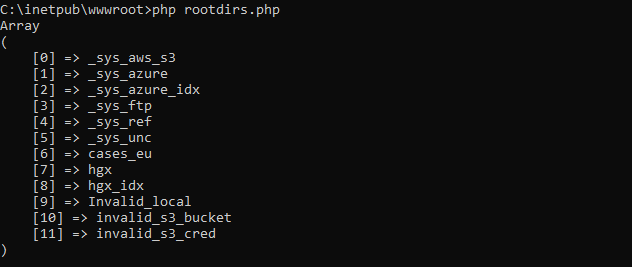
Bug spotting
Embedded in a Jupyter notebook, the output of the code looks like this:
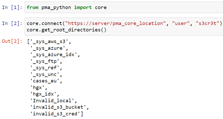
However, occasionally, people would tell us that the code mysteriously stopped working, and they were getting this:
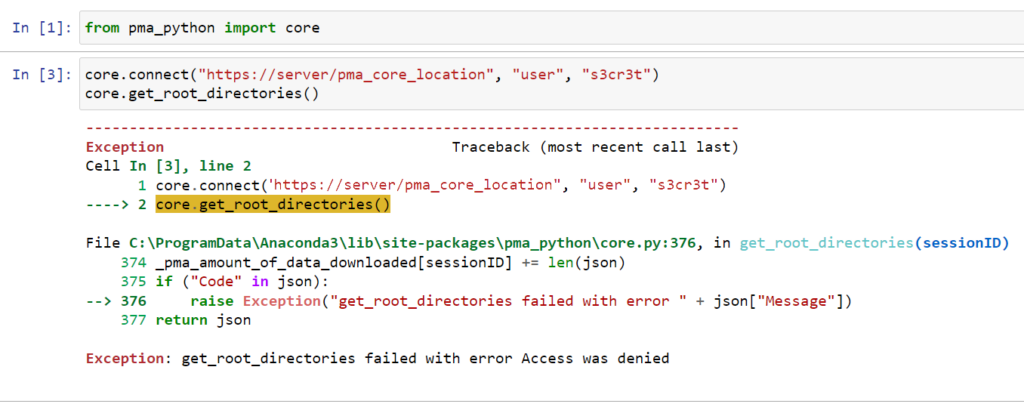
We couldn’t figure it out right away. It’s a typical “sometimes it works, sometimes it doesn’t”; the most frustrating kind of bugs.
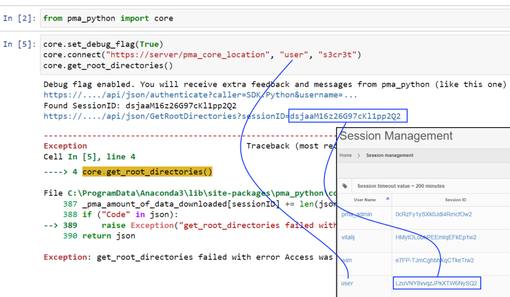
Almost by accident we found out what the problem was. By turning on the debug_flag, we get a better understanding of what’s happening.
As it turns out, the authentication call goes through just fine. But the SessionID passed on to the get_rootdirectories() API call, doesn’t match the returned sessionID from said original call.
Under the hood of the SDK
We designed the interface of the SDK for convenience. We want end-users to pick it up as quick as possible (keeping Larry Wall’s “laziness”, “impatience”, and “hubris” virtues in mind, too).
This means that once you connect to a PMA.core instance, and only a single PMA.core instance, you can pretty much ignore the returned SessionID value and just use the SDK functions with default arguments; the SDK is smart enough to figure out that there is only a single SessionID in play anyway, and retrieves that automatically from an internal HashMap-like cache, passing it on to when the eventual PMA.core API are invoked. It’s convenience, it’s how we thought we could make our interface programmer-friendly.
Intended use
The approach works find in a scripted scenario like Jupyter Python scripts, where you use a PMA.core SessionID for the duration of your script, and then you’re off doing something else again.
In different contexts however, like our AEM plugin (which in turn relies on the PMA.java SDK), it’s possible for a SessionID to be suspended in between subsequent SDK/API calls.
And that’s when the problem occurs.
The solution
The solution is relatively simple: it suffices to capture the returned SessionID from the authenticate call, and pass that on explicitly to subsequent methods. Like this:
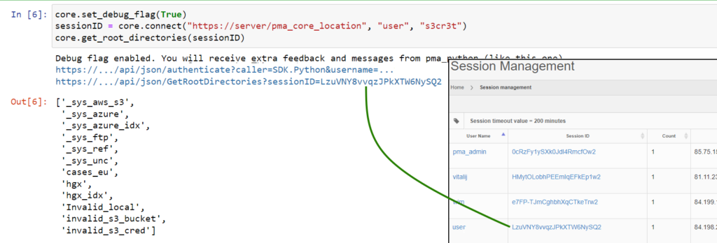
Now you can see that the SessionIDs match up, and the output remains as expected, even if the Session would be somehow terminated in the middle of the processing flow (as you as you keep re-authenticating at least).
Also note that in the back-end, the SDK now simply keeps track of two SessionID.
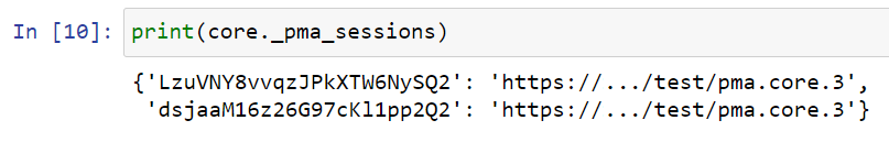
One of which is expired, which the SDK doesn’t know. But that’s all right, as long as you make sure that the correct SessionID is passed along explicitly.
How to upload your slides to PMA.core?
It’s a question people ask us all the time: How can I upload my slides to PMA.core? And usually we tell them: you don’t. You put the slides somewhere, point PMA.core to it by means of a root-directory, and that’s it: it’s the DP/WSI equivalent of What you see if what you get (WYSIWYG).
Sometimes this is insufficient. “But how can we still upload them?” is asked next, after we explain the concept of root-directories, mounting points, and other technicalities.
To be clear: Pathomation’s PMA.core tile server is NOT like the others: there is no registration mechanism, or upload procedure to follow. You really do drop your files off in a folder, and that’s it.
But it’s the dropping off that can be misconstrued as an “upload” procedure in itself. Instead, we prefer the term “transfer” instead. It’s also why we names one of our helper programs for this PMA.transfer.
Procedure
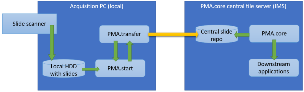
There are two scenario whereby slidetransfer is particularly relevant:
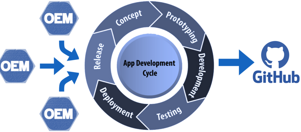
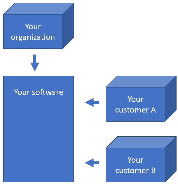
Within an organization, slide acquisition occurs on one computer, whereas the IMS solution runs on a centralized server. The challenge is to get the slides from the original acquisition PC to the central IMS (PMA.core tile server). The upload (or transfer) operation required is highlighted with the yellow arrow in the diagram below:
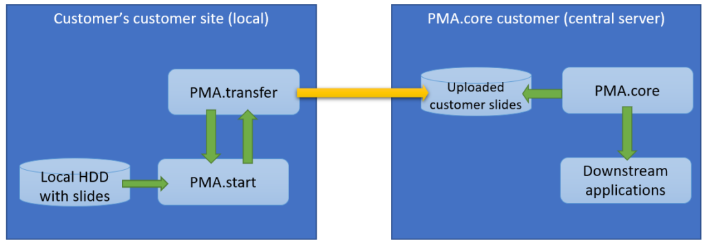
The second procedure is a variation of this; a PMA.core tile server customer has his own customers that want to transfer slides to a central repository for things like quality control or AI algorithms.
The scenario changes only a little and it’s mostly a matter of labels:
The latter is also known as a multi-tenant scenario. It’s possible to imagine for something like this to happen:
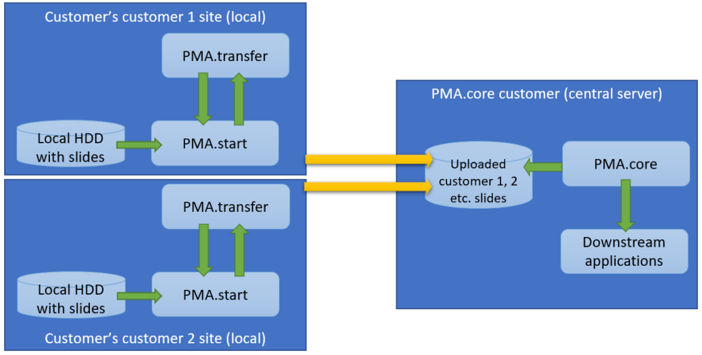
In the diagrams above we illustrate manual flow with PMA.transfer, but once this process becomes repetitive, it can be further automated by combining operating system functionality along with PMA.core SDK methods.
In this article, we present how to automate uploading your slides from the slide scanner PC to your PMA.core server (the first scenario).
Let’s have a look at how this could work in a Microsoft Windows environment.
File system auditing
The first step is to enable auditing to record when a user puts a new file in the folder you want to track. This user can be “Everyone” or a specific user, like the user that the slide scanner uses to output the digital slides.
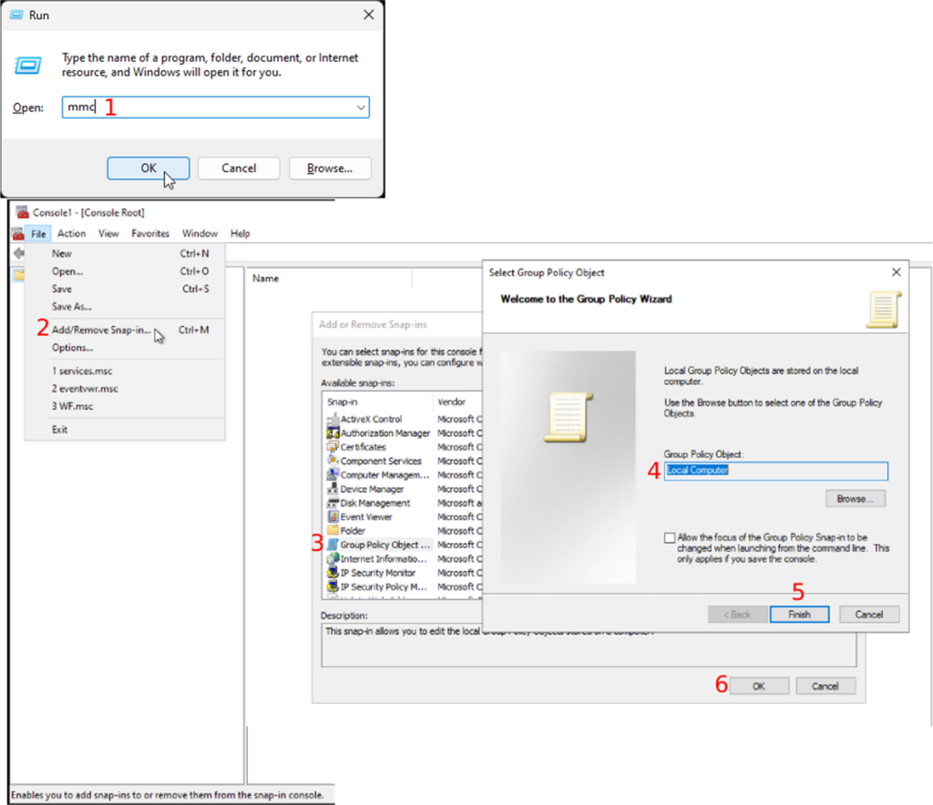
- Open the “Run” program using the shortcut “WIN + R”
- Enter “mmc” to open the Management console (Fig.1-1).
- Once the Management console is open, you will follow “File → Add/Remove Snap-in”
- Double-click on “Group Policy Object” in the “Available snap-ins” section
- Choose “Local Computer” as the “Group Policy Object”
- Continue by clicking on the “Finish” button
- Followed by the “OK” button
Continue on with the following steps:
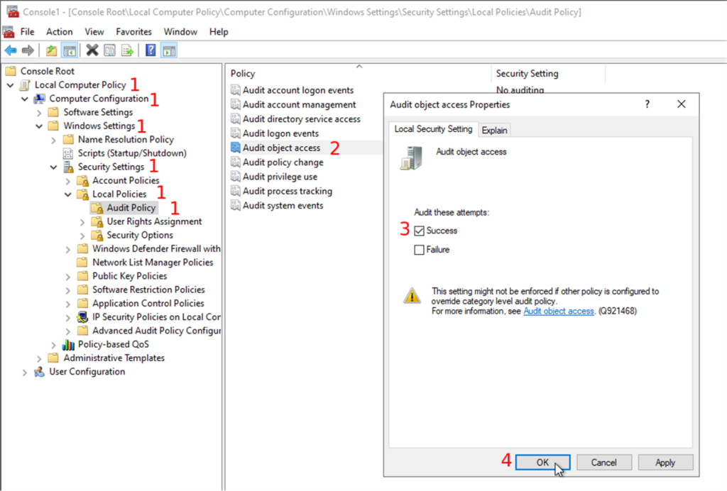
- Expand the “Local Computer Policy” and follow “Computer Configuration → Windows Settings → Security Settings → Local Policies → Audit Policy”
- Then, you will double-click on the object access audit in the list of audit policies
- Check the successful attempts checkbox in the properties window.
- You can also audit the failed attempts to do some error handling, but we will only focus on the successful attempts in this post.
- Confirm your changes by clicking on the “OK” button
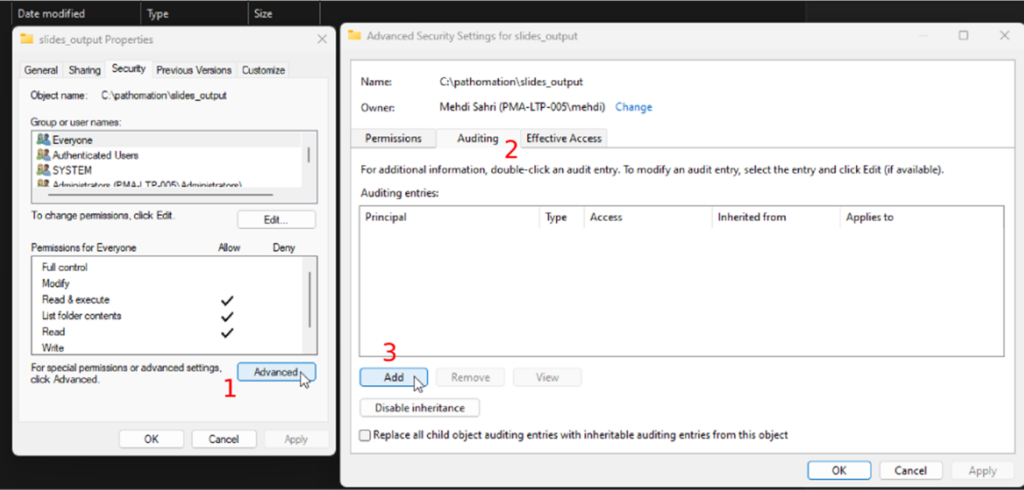
Now that you have the configuration correctly set up, you can enable audit trailing on the folder that you want to track (in other words: the folder where your whole slide images will be deposited).
- Go to the folder you want to track; this could be the folder where the slide scanner outputs the digital slides.
- Open the folder’s properties and the advanced security settings under the “Security” tab
- Next, you will open the “Auditing” tab
- Click on the “Add” button
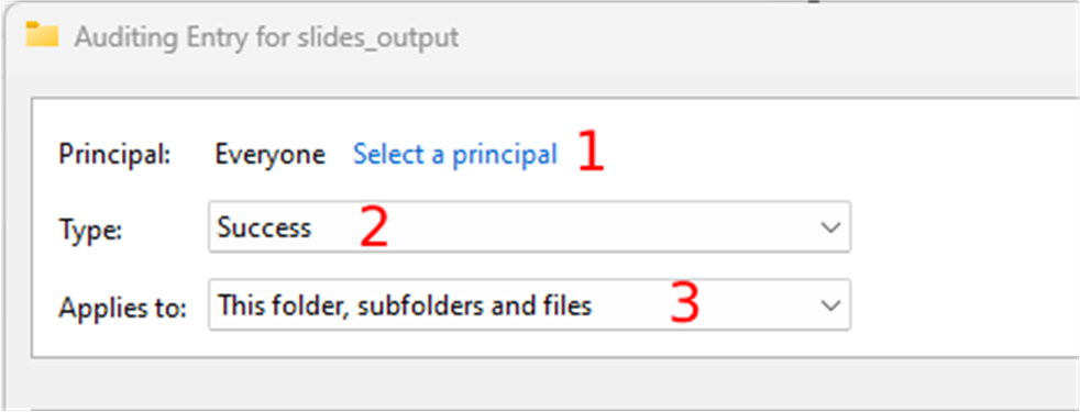
Next you can select the user that you want to track:
- Click on the “select a principal” link. This user can be “Everyone” or a specific user, like the user that the slide scanner uses to output the digital slides.
- Select the success type in the “Type” dropdown, and
- Choose the “This folder, subfolders, and files” option in the “Applies” dropdown
- Click on the “show advanced permissions” link in the permissions section and
- make sure only the “Create files / write data” checkbox is checked
- Confirm your changes by clicking all the OK buttons until the properties window closes
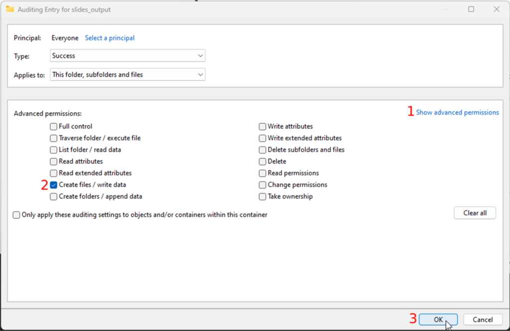
Congratulations; you will now be notified every time a new file (slide) is dropped in the folder.
The upload script
Let’s create the upload script. This script will be triggered to upload the slides to your PMA.core. Find the whole script at the end of this post.
First, you will import the needed packages. The only third-party package is the pathomation package. You can get it by running the “pip install pma_python” command in the command prompt.
There are three modules/packages used:
- os: This module will be used to perform file system actions.
- time: This module will be used to create timestamps, etc.
- pma_python: This package will be used to communicate with your PMA.core server.
The script uses timestamps, so only the recently added files get uploaded. First, it will check if the “date.txt” file exists and create it if it doesn’t. The “date.txt” file contains the timestamp of the last time the script ran. It gets read if it already exists. It gets created if it doesn’t exist, and the current timestamp gets written into it:
if os.path.exists(r"./date.txt"):
    last_timestamp = open('./date.txt','r')
    timestamp = last_timestamp.readlines()
    time.sleep(1)
    now = str(time.time())
    if timestamp[0] < now:
        print(timestamp[0] + ' ~ ' + now)
        last_timestamp = open('./date.txt','w')
        last_timestamp.write(now)
        check_connection(timestamp[0])
else:
    now = str(time.time())
    last_timestamp = open('./date.txt','w')
    last_timestamp.write(now)
    check_connection(5.5)

last_timestamp.close()
Once “date.txt” gets read or created, the “check_connection” function gets called with the timestamp or a low float number as the “last_trigger” argument. In this example, you will see that the “low float number” is “5.5”. This low float number ensures that the files in the folder get uploaded if the “date.txt” file does not exist.
The “check_connection” function checks if PMA.start is running and if you have a valid session id. If they are both true, the “last_trigger” argument gets passed to the “upload_files” function. You can expand the “check_connection” function to automatically run PMA.start, try other credentials, send emails, etc.
def check_connection(last_trigger):
    sessionID = core.connect('https://snapshot.pathomation.com/PMA.core/3.0.1', 'pma_demo_user', 'pma_demo_user')

    if core.is_lite() and sessionID is not None:
        print("PMA.start is running")
        upload_files(sessionID, last_trigger)
    else:
        print("PMA.start is not running")
        input("Press Enter to continue...")
In the “upload_files” function, you check and upload the recently added files to your PMA.core.
<code class="python"><pre>
supported_files = [".jpeg", ".jpg", ".jp2", ".png", ".vsi", ".dzi", ".vms", ".ndpi", ".ndpis", ".dcm", ".mrxs", ".svs", ".afi", ".cws", ".scn", ".lif", "DICOMDIR", ".zvi", ".czi", ".lsm", ".tf2", ".tf8", ".btf", ".ome.tif", ".nd2", ".tif", ".svslide", ".ini", ".mds", ".zif", ".szi", ".sws", ".qptiff", ".tmap", ".jxr", ".kfb", ".jp2", ".isyntax", ".rts", ".rts", ".bif", ".zarr", ".tiff", ".mdsx", ".oir"]
…
def upload_files(sessionID, last_trigger):
    list_content = os.listdir(os.getcwd())

    for list_item in list_content:
        if os.path.isfile(list_item):
            root, ext = os.path.splitext(list_item)
            if ext in supported_files:
                creation_file = os.path.getctime(list_item)
                if float(last_trigger) < creation_file:
                    print('Uploading S3...')
                    core.upload(os.path.abspath(list_item), "_sys_aws_s3/testing_script", sessionID, True)
            else:
                print(list_item, 'is not supported')
</pre></code>
First, all the objects i.e. files and directories in the tracked folder, get put into the “list_content” array. A for loop loops over all the items and performs a couple of checks to get the recently added files. The first check checks if the item in the “list_content” array is a file. This blocks directories from being uploaded.
list_content = os.listdir(os.getcwd())

    for list_item in list_content:
        if os.path.isfile(list_item):
Next, the file path gets split into 2 parts: The file’s root and the file’s extension. The file’s extension gets compared with the “supported_files” array to ensure that only supported files get uploaded to your PMA.core.
supported_files = [".jpeg", ".jpg", ".jp2", ".png", ".vsi", ".dzi", ".vms", ".ndpi", ".ndpis", ".dcm", ".mrxs", ".svs", ".afi", ".cws", ".scn", ".lif", "DICOMDIR", ".zvi", ".czi", ".lsm", ".tf2", ".tf8", ".btf", ".ome.tif", ".nd2", ".tif", ".svslide", ".ini", ".mds", ".zif", ".szi", ".sws", ".qptiff", ".tmap", ".jxr", ".kfb", ".jp2", ".isyntax", ".rts", ".rts", ".bif", ".zarr", ".tiff", ".mdsx", ".oir"]
…
root, ext = os.path.splitext(list_item)
            if ext in supported_files:
The last check compares the “created on” timestamp of the file with the “last_trigger” argument that got passed on from the “check_connection” function. The upload starts if the “created on” timestamp is bigger than the “last_trigger” argument using the “core.upload()” function. The arguments of the “core.upload()” function are:
- local_source_slide: This is the absolute path of the file.
- target_folder: This is the PMA.core folder you want to upload to.
- target_pma_core_sessionID: This is the session id you created in the “check_connection” function.
- callback=None: This argument will print the default progress of the upload if set to True. You can also pass a custom function that will be called on each file upload. The signature for the callback is “callback(bytes_read, bytes_length, filename)”.
creation_file = os.path.getctime(list_item)
                if float(last_trigger) < creation_file:
                    print('Uploading S3...')
                    core.upload(os.path.abspath(list_item), "_sys_aws_s3/testing_script", sessionID, True)
Save the script and put it in the track folder.
Create a scheduled task
In this last step, you will create a scheduled task in the Task Scheduler to run the script when the scanner outputs the digital slides in the track folder.
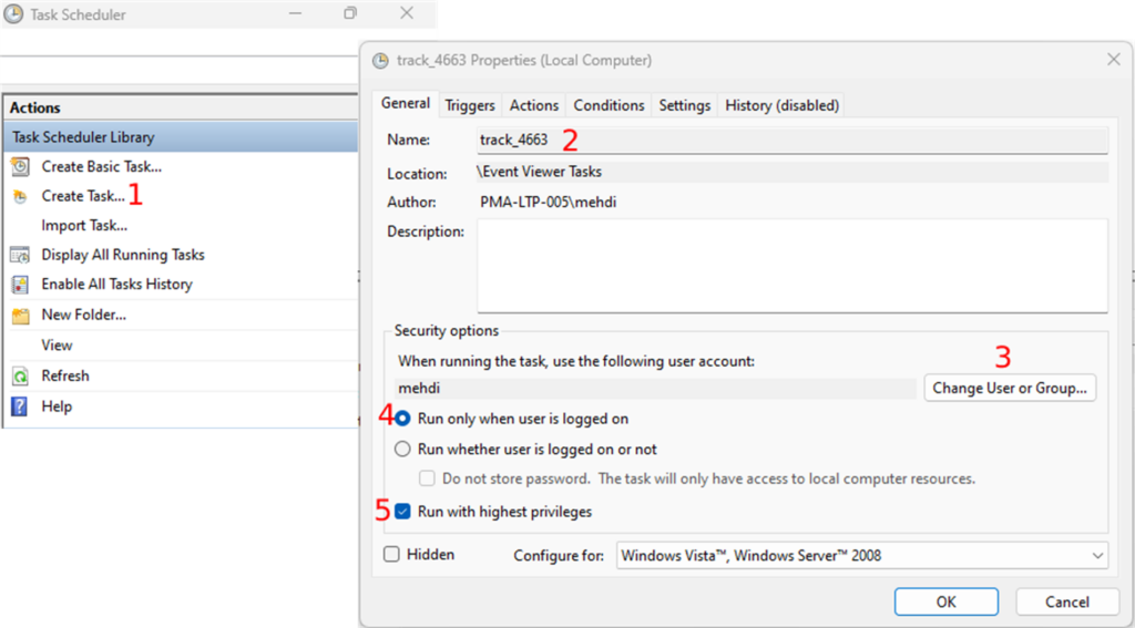
- Open the Task Scheduler and click on “Create Task” in the “Actions” section
- Under the “General” tab, enter the name of the task and
- Choose a user in the “Security options” section. You do this by clicking on the “Change User or Group” button (Fig.6-3). This is the slide scanner user that outputs the digital slides in the track folder. You can keep the default user if the current user stays logged on.
- Next, you will select the “Run only when user is logged on” radio button (Fig.6-4) and
- Check the “Run with highest privileges” checkbox (Fig.6-5).
Under the “Triggers” tab, you can now create the task’s trigger by clicking on the “New” button:
- In the “Begin the task” dropdown, you will select what the trigger will listen to.
- You will choose the “On an event” option, and
- Select the “Custom” radio button.
- Click on the “New Event Filter” button, and
- Go to the “XML” tab. Under the “XML” tab, you will check the “Edit query manually” checkbox
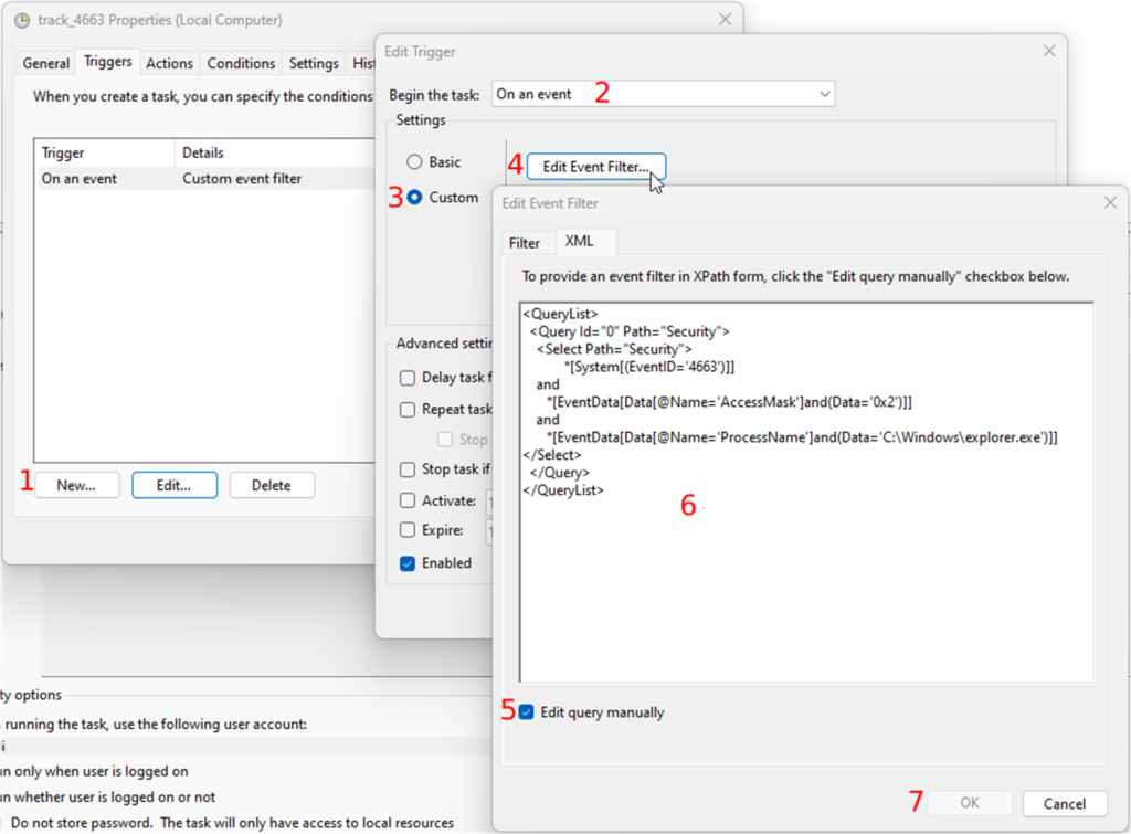
Paste the following XPath code:
<QueryList>
  <Query Id="0" Path="Security">
    <Select Path="Security">
            *[System[(EventID='4663')]]
    and
       *[EventData[Data[@Name='AccessMask']and(Data='0x2')]]
    and
       *[EventData[Data[@Name='ProcessName']and(Data='C:\Windows\explorer.exe')]]
</Select>
  </Query>
</QueryList>
Confirm all your changes by clicking on the OK button until you get to the “Create Task” window.
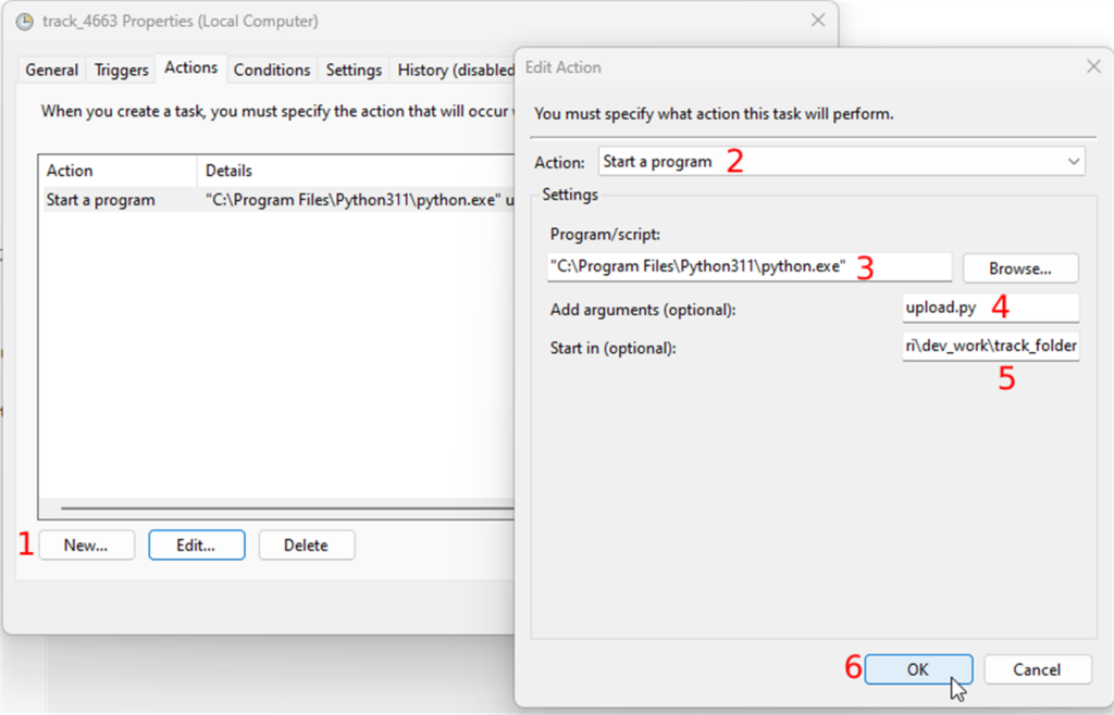
The next tab is “Actions”. The task will perform this action when the event occurs. The action here is running the script in the track folder. To create an action you
- Click on the “New” button and
- Select “Start a program” in the “Action” dropdown
- In the “Settings” section, you will browse the python executable which should be in "C:\Program Files\Python311\python.exe", and
- In the “Add arguments” field you will enter the name of the script with the “.py” extension.
- Finally, you enter the path of the track folder in the “Start in” field and
- Confirm your changes by clicking the OK button.
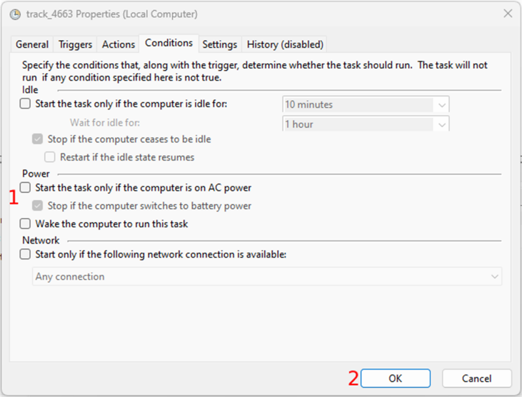
The second to last tab is “Conditions”. The only thing you need to do here is to uncheck all the checkboxes in the “Power” section
Finally, you can create the task by clicking on the “OK” button. You can test the task by selecting the task and clicking on “Run” in the “Selected Item” section. This should run the script in the track folder.
The full script:
import os
import time
from pma_python import core

supported_files = [".jpeg", ".jpg", ".jp2", ".png", ".vsi", ".dzi", ".vms", ".ndpi", ".ndpis", ".dcm", ".mrxs", ".svs", ".afi", ".cws", ".scn", ".lif", "DICOMDIR", ".zvi", ".czi", ".lsm", ".tf2", ".tf8", ".btf", ".ome.tif", ".nd2", ".tif", ".svslide", ".ini", ".mds", ".zif", ".szi", ".sws", ".qptiff", ".tmap", ".jxr", ".kfb", ".jp2", ".isyntax", ".rts", ".rts", ".bif", ".zarr", ".tiff", ".mdsx", ".oir"]

def check_connection(last_trigger):
    sessionID = core.connect('pma_core_url’, 'pma_core_username', 'pma_core_pw')

    if core.is_lite() and sessionID is not None:
        print("PMA.start is running")
        upload_files(sessionID, last_trigger)
    else:
        print("PMA.start is not running")
        input("Press Enter to continue...")

def upload_files(sessionID, last_trigger):
    list_content = os.listdir(os.getcwd())

    for list_item in list_content:
        if os.path.isfile(list_item):
            root, ext = os.path.splitext(list_item)
            if ext in supported_files:
                creation_file = os.path.getctime(list_item)
                if float(last_trigger) < creation_file:
                    print('Uploading S3...')
                    core.upload(‘local_source_slide’, ‘target_folder’, ‘target_pma_core_sessionID’, callback=None)
            else:
                print(list_item, 'is not supported')


if os.path.exists(r"./date.txt"):
    last_timestamp = open('./date.txt','r')
    timestamp = last_timestamp.readlines()
    time.sleep(1)
    now = str(time.time())
    if timestamp[0] < now:
        print(timestamp[0] + ' ~ ' + now)
        last_timestamp = open('./date.txt','w')
        last_timestamp.write(now)
        check_connection(timestamp[0])
else:
    now = str(time.time())
    last_timestamp = open('./date.txt','w')
    last_timestamp.write(now)
    check_connection(5.5)

last_timestamp.close()
Conclusion
In this article we looked at how you can gradually convert manual slide transfer workflows over to automated ones.
After you implement the steps and code from this program, you will be able to deposit slides in an audit-trailed folder on your hard disk, and subsequently be transferred to your PMA.core tile server (for testing purposes these can even reside on the same machine).
We wrote the code in this article from the point of view of Microsoft Windows, and we used the Python scripting language as glue. But other combinations are possible. Let us know if there's a particular scenario that you would like to see explored in a follow-up article.
Key to this procedure is the SDK's Core.upload() method. This is really where all the magic happens. In a subsequent article, it is our intention to offer a comparison look between how this particle method (and its Core.download() counterpart) functions in each of the respective language platforms we support: Python, Java, and PHP.
Multi-tenant with PMA.core and PMA.vue
In our recent posts, we’ve talked a lot about PMA.studio and high-end topics in digital pathology like AI and upload automation workflows.
In this article, we want to discuss a more mundane scenario, whereby you are a pathology service provider (or maybe a group practice).
Multi-tenant
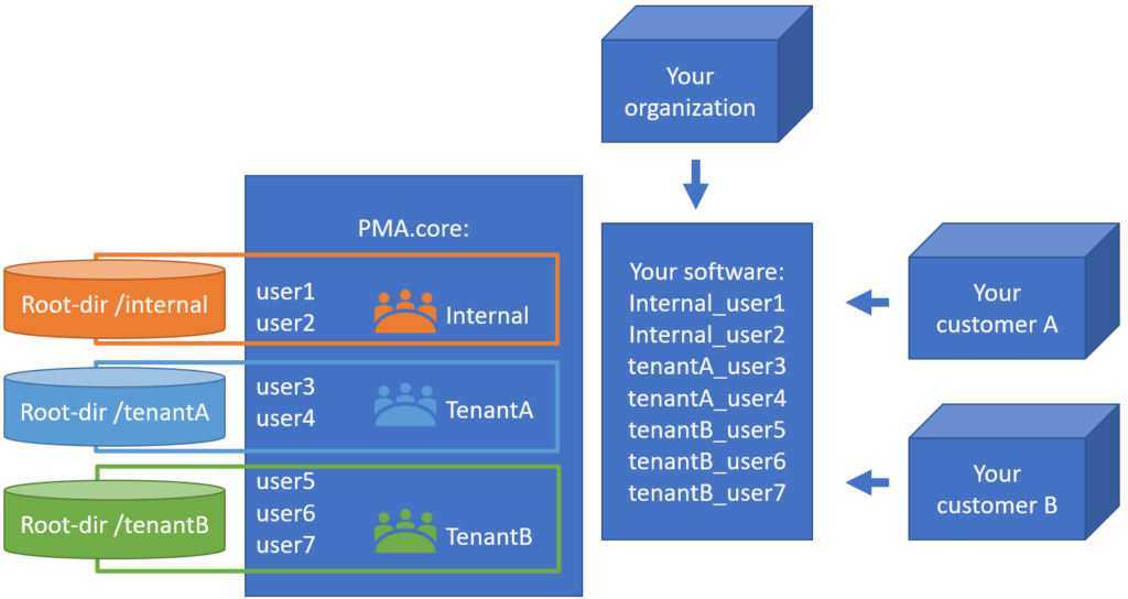
Simply put and for our purposes: a multi-tenant scenario is where you have a single software installation, with different users from different origins. Your users don’t just make up the internal users within your own organization; they represent your customers as well.
Typical of a multi-tenant environment is that each tenant may have vastly different interests. Regardless, each tenant is very keen on its own privacy, and so its paramount that tenant A under no circumstances can see the content of tenant B.
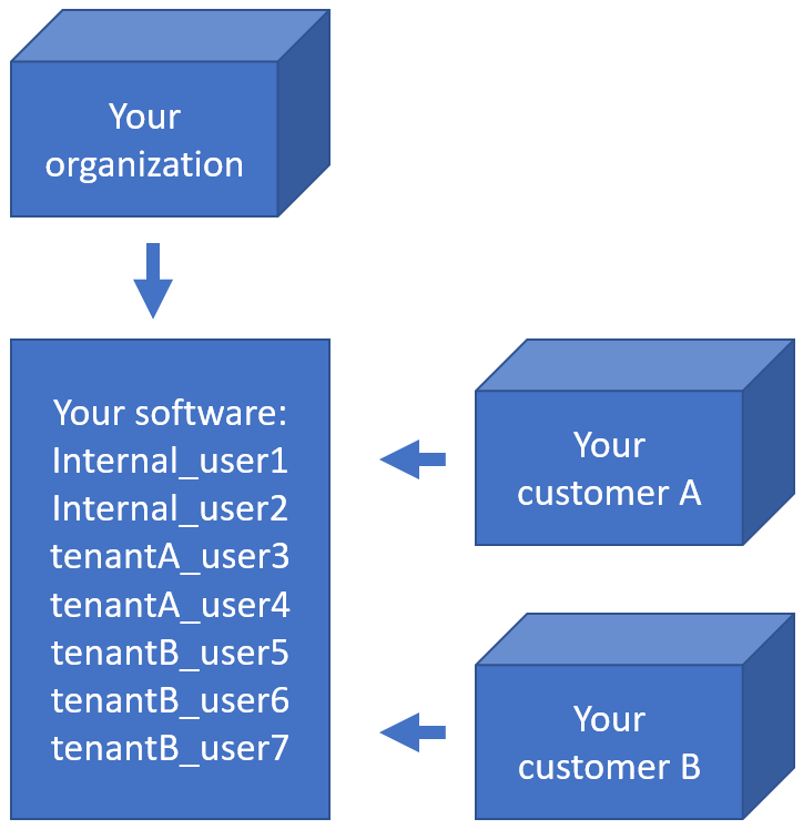
Suppose you have a total of 7 actual users (representing physical persons), they may be distributed across your tenants and your own organization like this:
How do you deal with that?
Let’s look how do PMA.core and PMA.vue help you achieve pathology exchange nirvana.
PMA.core security provisions
Let’s start with the obvious one: security. Keeping the data from your own organization separate from your customers is achieved by defining separate root-directories and users in PMA.core.
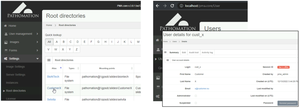
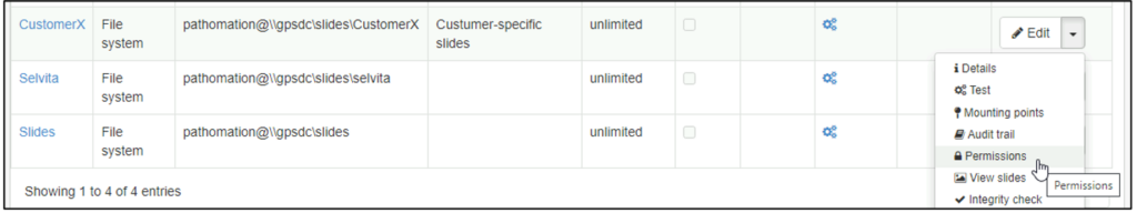
Once you’ve defined both users and root-directories, you can use PMA.core’s built-in access control rights (ACL) to control who gets to see what.
As your own customer-base grows (because you’re using this awesome Pathomation software!) you can create groups as well, and organize your customer-accounts accordingly.
Once the accounts, root-directories and credentials are configured, you can go to PMA.vue. A tenant user that logs in, will only be able to see the tenant-specific slides. There is no way see the other tenant’s slides, either on purpose or by accident.
What about your own users?
You can set permissions on the various root-directories so that your internal users at least can have access to the respective tenant slides that they have to interact with. You could even go more granular so that internal users only have access to select tenants, based on the specific terms of for SoWs and MSAs. For tenant users themselves nothing changes because of this: they still can only their own slides.

Licensing PMA.core
Once people are convinced that our security model can fit their deployment scenarios, the next question is usually about licensing.
You don’t have to buy PMA.core licenses for all the your tenant users. It is typical for a tenant to have at least two user accounts: a primary and a backup (for when the original user is out, or on vacation or so).
PMA.core wotks with concurrent roaming licenses. This means that in the above scenario, you would only buy a single roaming seat license to accommodate access for TenantA’s users at any given time.
It gets better actually: when it’s unlikely that all of your tenants will be using your system at the same time, you can distribute the seats amongst all the tenants (as well as your internal users) together.
Let’s have a look at the following scenario: you run a small group practice with 5 pathologists, and have 20 tenants. Reading the slides typically happens overnight, and during the daytime, you estimate that about a fourth of your customer base at any given time would be uploading new content to you using PMA.transfer, and another fourth consulting analytical results. Consulting results typically happens in the morning, uploading new content in the afternoon.
Your seat occupation would therefore be about 5 users at night, about 5 users in the morning (one fourth of 20 tenants), and 5 users in the afternoon (one fourth of 20 tenants again).
So even as you have a total or 20 (tenants) x 2 (primary, backup) + 5 (internal staff) = 45 people interact with your system, at any given time you would provision 5 simultaneously occupied seats. Let’s just add one more to that number to be sure, because you may occasionally also need parallel administrative access, maybe an extra hand helps out on busy days etcetera.
You can configure PMA.core to send out automatic notification email should the number of concurrent licenses is insufficient at any given time. Do you notice at some point that you are effectively short on seats? Not a problem; contact us to purchase additional roading license seats at any given time, and we can send you an updated license key file right away.
More information about our licensing policy (and latest updates) can be found at https://www.pathomation.com/licensing/.
PMA.vue
PMA.vue is Pathomation’s lightweight centralized viewing solution. Like PMA.core, it can be installed on-premise on your end, or hosted by us on a Virtual Machine in a data center of your choice (currently we support Amazon AWS and Microsoft Azure).

With PMA.vue, you can offer powerful viewing and basic annotation capabilities, without having to compromise PMA.core itself: all registered PMA.core users can access PMA.vue, but not vice versa: in order to be allowed to log into PMA.core, a special attribute must be enabled for the user.
With PMA.vue, you can extend slide viewing features to your tenant users, without to need to invest into having your own customer portal developed. Tenants can look at slides, create screenshots, prepare publications etcetera. For your own internal employees, PMA.vue has a whole arsenal of data sharing options. So even if you don’t open up PMA.vue to tenant users, it is still a great tool for internal communication, as you can use it to share folders, slides, and even regions of interest.
Learn more?
To learn more about PMA.vue, visit https://www.pathomation.com/pma.vue
To learn more about PMA.core, visit https://www.pathomation.com/pma.core
Not sure about whether you should go with PMA.vue or build your own customer portal (using our SDK and PMA.UI visualization framework)? We have a separate blog article to help you decide who to put in the driver seat.
Quod AI (What about AI)?
A few months ago we published a blog article on how PMA.studio could be used as a platform in its own right to design bespoke organization-specific workflow and cockpit-solutions.
In the article we talked about LIMS integration, workflow facilitation and reporting.
We didn’t talk about AI.

We have separate articles though in which we hypothesize and propose how AI – Pathomation platform integration could work; see our YouTube videos on the subject.
So when we recently came across one AI provider with a stable and well documented API, we jumped at the opportunity to pick up where we left off: and we built an actual demonstrator with PMA.studio as a front-end, and the AI engine as a back-end engine.
AI and digital pathology
At a very, very, VERY high level, here’s how AI in digital pathology works:
- The slide scanner takes a picture of your tissue at high resolution and stores it on the computer. The result of this process is a whole slide image (WSI). So when you look at the whole slide images on your computer, you’re looking at pixels. A pixel is very small (about 2 – 3 mm on your screen, if you really have to know).
- You are a person. You look at your screen and you don’t see pixels; they blend together to see images. If you’ve never looked at histology before, WSI data can look like pink and purple art. If you’re a biology student, you see cells. If you’re a pathologist, you see tumor tissue, invasive margins, an adenocarcinoma or DCIS perhaps.
- The challenge for the AI, is make it see the same things that the real-life person sees. And it’s actually much harder than you would think: for a computer program (algorithm), we really start at the lowest level. The computer program only sees pixels, and you have to teach it somehow to group those together and tell it how to recognize features like cells, or necrotic tissue, or the stage of cell-division.
It’s a fascinating subject really. It’s also something we don’t want to get into ourselves. Not in the algorithm design at least. Pathomation is not an AI company.
So why talk about it then even at all? Because we do have that wonderful digital pathology software platform for digital pathology. And that platform is perfectly suited to serve as a jumping board to not only rapidly enrich your LIMS with DP capabilities, but also to get your AI solution quicky off the ground.
If you’re familiar with the term, think of us a PaaS for AI in digital pathology.
Workflow
In one of our videos, we present the following abstract workflow:
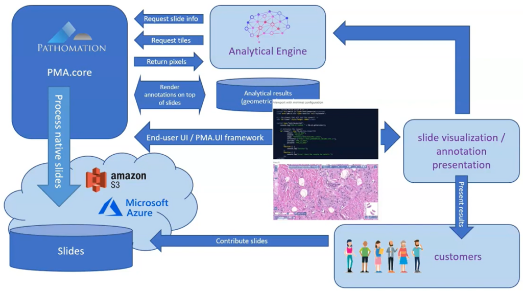
Now that we’ve established connections to an AI providers ourselves, we can outline a more detailed recipe with specific steps to follow:
- Indicate your region(s) of interest in PMA.studio
- Configure and prepare the AI engine to accept your ROIs
- Send off the ROI for analysis
- Process the results and store them in Pathomation (at the level of PMA.core actually)
- Use PMA.studio once again to inspect the results
Let’s have a more detailed look at how this works:
Step 1: Indicate your regions of interest
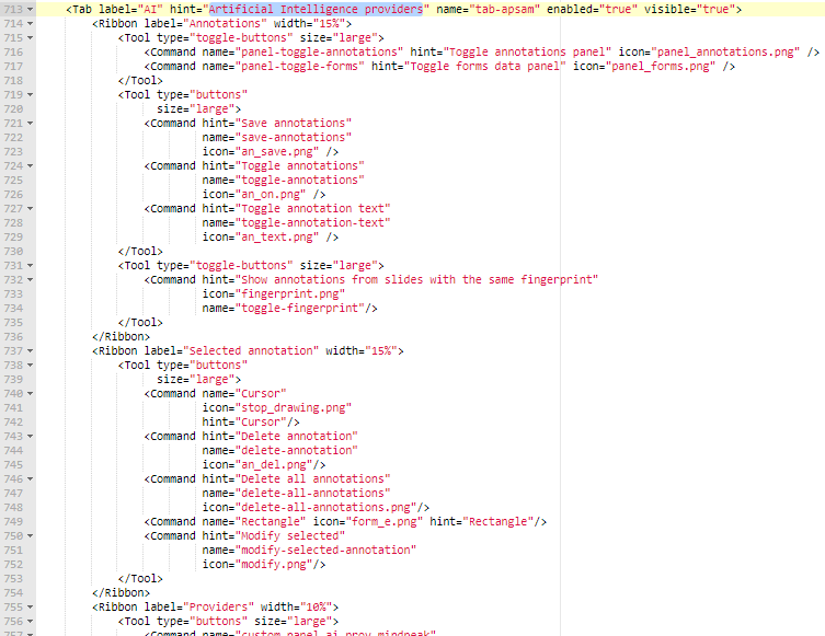
With the rectangle tool on the Annotations tab of the ribbon, you can draw a region of interest.
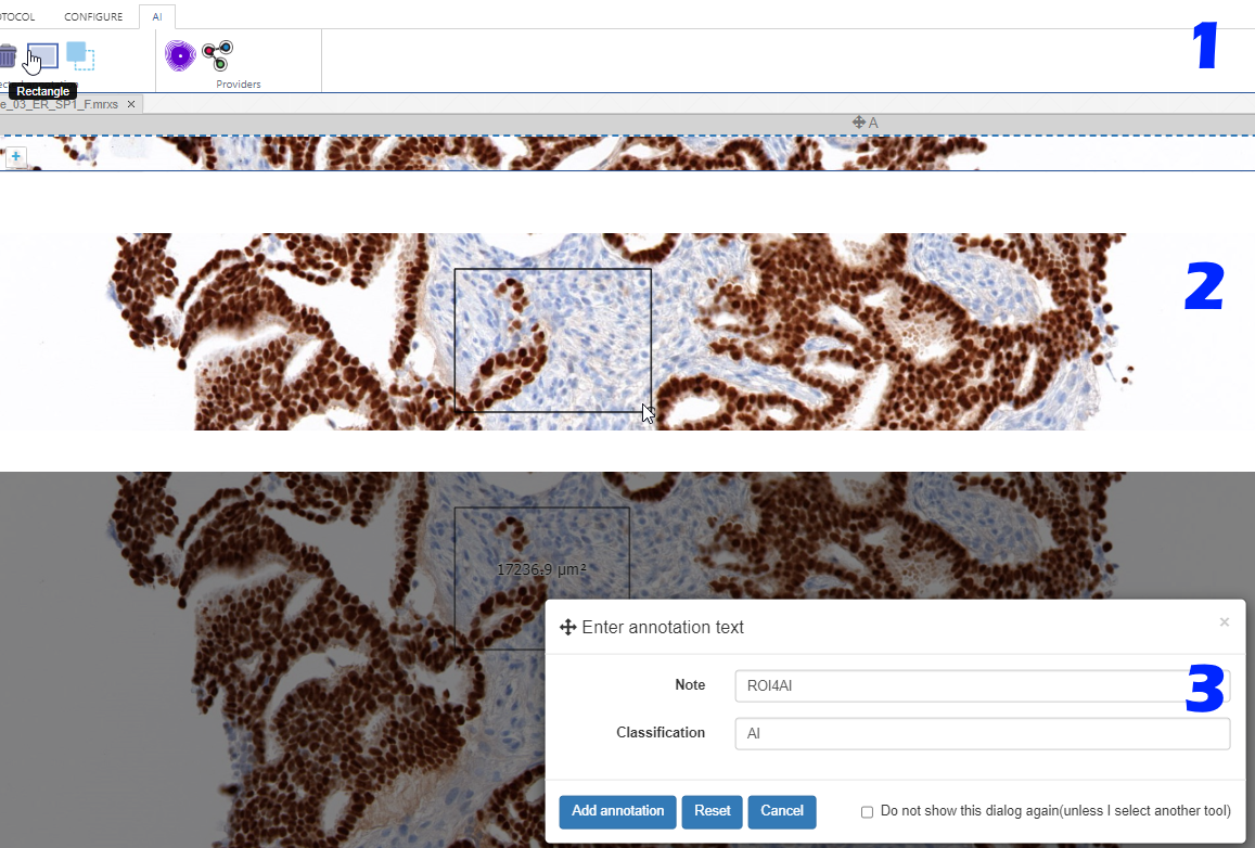
Don’t worry about the resolution (“zoomlevel”) at which you make the annotation; we’ll tell our code later on to automatically extract the pixels at the highest available zoomlevel. If you have a slide scanned at 40X, the pixels will be transferred as if you made the annotation at that level (even though you made have drawn the region while looking at the slide in PMA.studio in 10X).
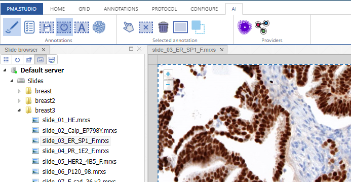
You can actually configure a separate AI-tab in the back-end of PMA.studio, and repeat the most common annotation tools you’ll use to indicate your regions of interest: if you know you’ll always be drawing black rectangular regions, there’s really no point having other things like compound polygon or a color selector:
Step 2: Configure the AI engine for ingestion
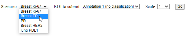
We added buttons to our ribbon to interact with two different AI engines.
When clicking on one of these buttons, you can select the earlier indicated region of interest to send of for analysis, as well as what algorithm (“scenario” in their terminology) to run on the pixels:
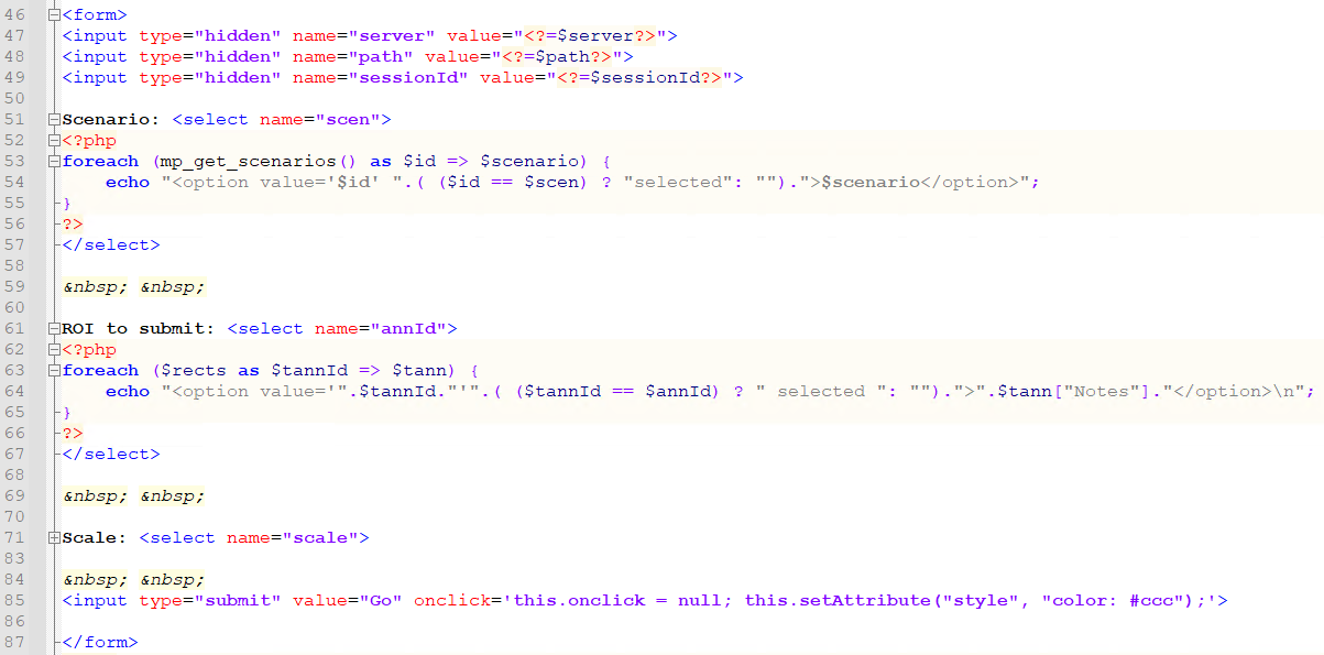
The way this works behind the scenes: the panel that’s configured in the ribbon ends up loading a custom PHP script. Information about the current slide in PMA.studio is passed along through PMA.studio’s built-in mechanism for custom panels.
The first part of the script than interacts both with the AI provider to determine which algorithms are available, as well as with the Pathomation back-end (the PMA.core tile server that hosts the data for PMA.studio) to retrieve the available ROIs:
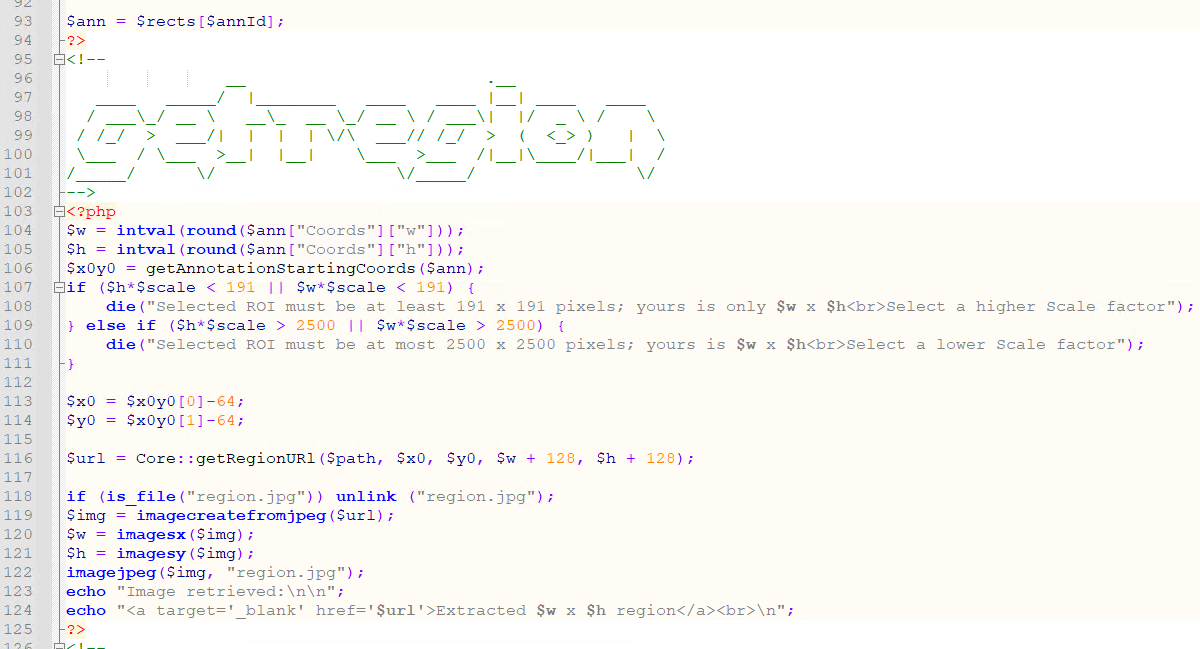
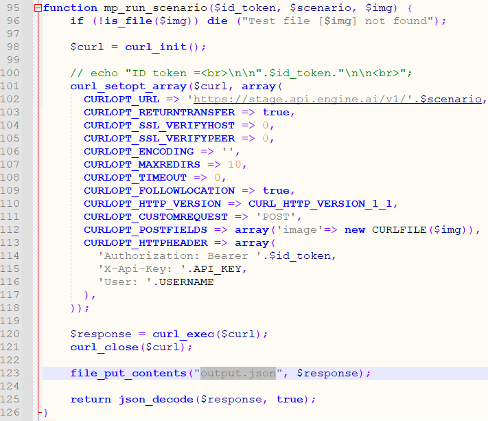
Step 3: Extract the pixels from the original slide, and send them off the AI engine
First, we use Pathomation’s PMA.php SDK to extract the region of pixels indicated from the annotated ROI:
We store a local copy of the extracted pixels, and pass that on to the AI engine, using PHP’s curl syntax:
Step 4: Retrieve the result and process it back into PMA.core
Finally, the returned JSON syntax from the AI engine is parsed and translated (ETL) into PMA.core multipoint annotations.
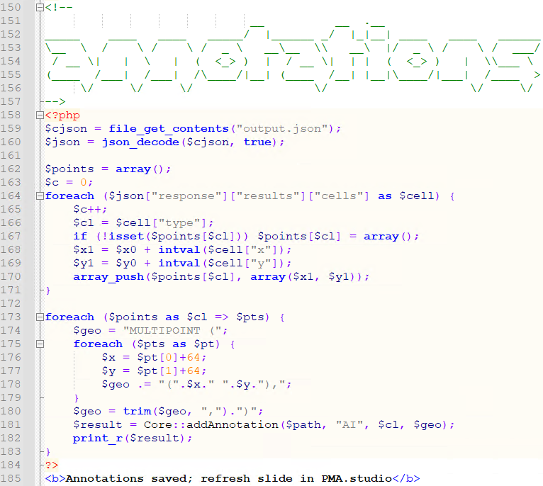
A form is also generated automatically to keep track of aggregate data if needed:

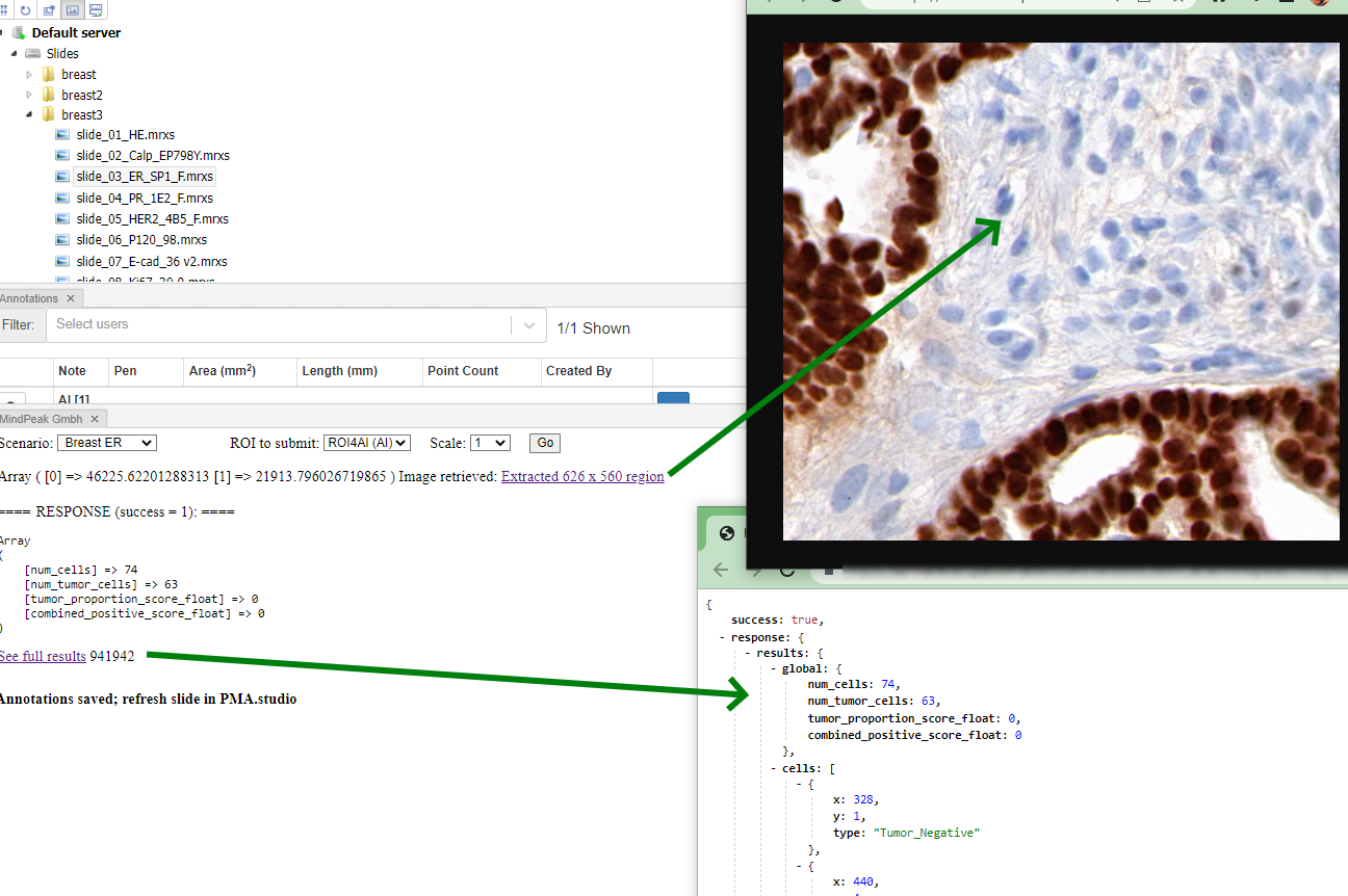
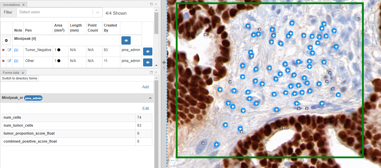
Step 5: Visualize the result in PMA.studio
The results can now be shown back into PMA.studio.
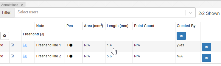
The data is also available through for the forms panel and the annotations panel:
What’s next?
How useful is this? AI is only as good as what people do with it. In this case: it’s very easy to select the wrong region on this slide where a selected algorithm doesn’t make sense to apply in the first place. Or what about running a Ki67 counting algorithm on a PR stained slide?
We’re dealing with supervised AI here, and this procedure only works when properly supervised.
Whole slide scaling is another issue to consider. In our runs, it takes about 5 seconds to get an individual ROI analyzed. What if you want to have the whole slide analyzed? In a follow-up experiment, we want to see if we can parallelize this process. The basic infrastructure at the level of PMA.core is already there.
Demo
The demo described in this article is not publicly available, due to usage restrictions on the AI engine. Do contact us for a demonstration at your earliest convenience though, and let us show you how the combination of PMA.core and PMA.studio can lift your AI endeavors to the next level.
An in-depth look at polygon annotations in PMA.studio
We’re all familiar with basic annotation patterns like rectangles, circles, lines etcetera. Pathomation’s PMA.studio support all of the through the “Simple shapes” panel on the Annotations tab:
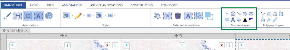
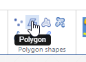
Next to this tab, a more interesting group is shown: polygon shapes. The various icons on these come from the unique way pathologists typically make their annotations.
In this article, we’re going to distinguish between all 7 buttons in the “polygon shapes” group.
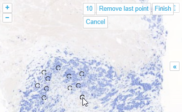
Multi point
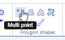
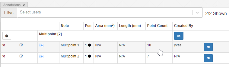
With the multi-point annotation you can quickly annotate a great amount of individual cells. A counter runs along as you indicate additional landmarks, and it is always possible to revert back on the latest annotated point.
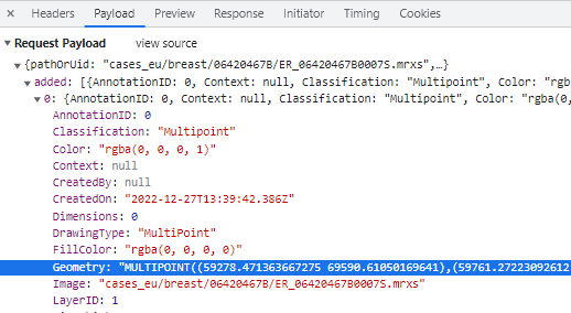
In WKT, the annotations are stored as “MULTIPOINT((x1 y1),(x2 y2),…” strings
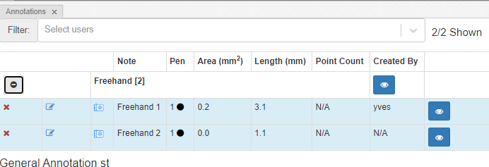
You can (of course) make multiple multi-point annotations. An overview is always available via the Annotations panel:
Polygon
Drawing polygon is the typical run off the mill polygon annotation tool you find in many graphics tools like Photoshop, Paint.Net etcetera. The tool, as implemented, assumes there’s an automatic connection between your first and last drawn point. You finish drawing your shape by double-clicking (unlike the multi-point tool, where you need to press an explicit “Finish” button).
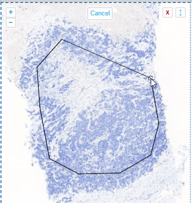
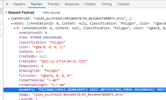
In WKT, polygons are stored as POLYGON((x1 y1,x2 y2,x3 y3,…,x1 y1)) strings. This means that when you have a polygon with 4 points, the WKT representation of it will actually indicate 5 points (the first and last one being the same).
The annotation browser this time doesn’t indicate of how many points the polygon shape is comprised.
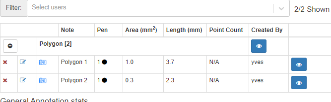
The annotation browser this time doesn’t indicate of how many points the polygon shape is comprised.
Closed freehand
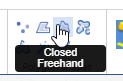
The closed freehand results is a kind of polygon shape annotation, but this time you keep the mouse button pressed down during the whole process of drawing the shape.
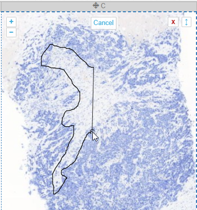
It’s best suited to annotate small areas at high magnification, possibly in combination with an alternative pointing device like a stylus (instead of a mouse).
Like the earlier mentioned polygon (and as the name suggests), the closed freehand is a closed form. It’s equally stored as a WKT POLYGON string:
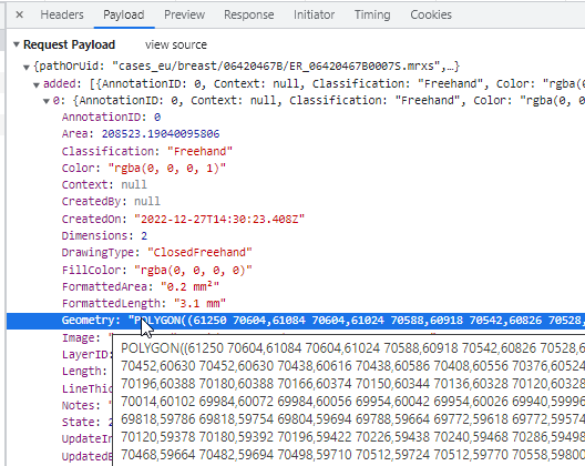
Because it’s a closed form, the annotation browser can determine both its area and surface:
Compound freehand

Right; this is one we’re particularly proud of. What’s the problem with annotating tissue regions? Sometimes you can do it at a coarse resolution, but sometimes you need a finer (higher) resolution, to indicate the exact border between two tissue types. A magic wand tool could work, but not always.
What you want to do in these cases is pan and zoom in and out a couple of times while tracing the border of your shape. But all modes of interaction with your mouse are already taken with conventional tools like polygon and closed freehand.
So the compound freehand gives you exactly that option: you can trace a boundary one segment at the time.
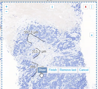
You zoom in and out, and pan as needed.
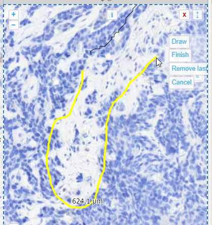
When you feel you have enough line segments drawn to delineate your entire area of interest, you press the “Finish” button, and all segments are joined into a single one.
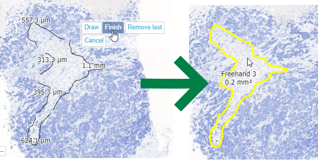
From a technical perspective, this is a PMA.UI front-end feature only (albeit a cool one!). Once completed and saved to PMA.core, the WKT representation is the same boring POLYGON:
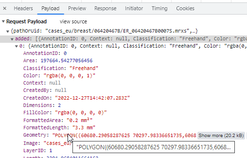
Why is this relevant? Because this means that once the different line segments are merged, it is not possible to pry them apart again into their origins.
Freehand
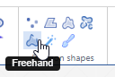
The freehand tool lets you draw an arbitrary line to indicate a margin.
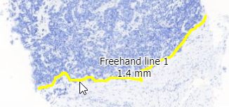
The way this is stored in WKT this time is by means of a LINESTRING. The final point can be whatever it is; it does not automatically revert back to the origin (that would make it a closed freehand).
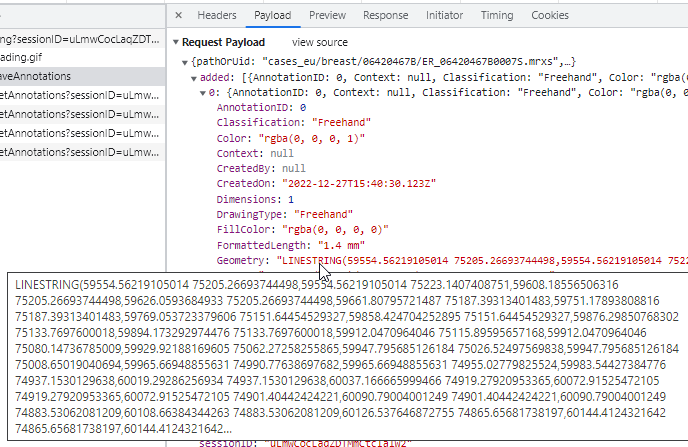
Because it’s a line this time, it’s only 1-dimensional, so there are no area measurements to display (none that would make sense anyway).
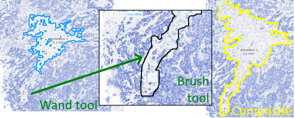
Wand
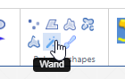
We refuse to call our wand “magic”, like in other environments. Think of our wand more as a magnetic lasso (which is another indication used oftentimes for similar tools).
The wand tool can be useful to select large regions with homogeneous coloring schemes, but we think it actually has limited use in histology and pathology. There are a number of reasons for this: Oftentimes what you really want is cell segmentation (e.g. highlight all the Ki67-positive cells), but a wand tools is not smart enough for that; it only acts on neighboring pixels (and based of the difference between already selected pixels, decides whether the next pixel is to be included or not).
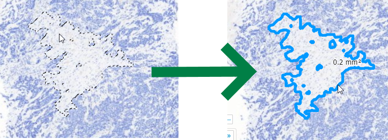
Our tool can still be useful to select lumens, or perhaps regions of fatty tissue. We’re including it at least in part because people have asked us for it. Like rectangles and circles, people sort of expect it (but tell us the last time you used a rectangle or indicate a cell or a region of interest… nature just doesn’t work that way).
The Wand tool therefore is probably one of the more experimental tools we have in our arsenal. Our best advice it to play around with it a bit and see if it’s useful in your particular observations. You can tweak it and set a couple of different parameters to change its sensitivity, as well. Use it at your discretion, and let us know how we can make it work (better) for you in a subsequent version of PMA.studio.
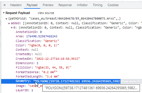
As with our compound polygon (cf. supra), technically speaking the Wand is a client-side tool. At the end of the day, it translates like all polygon-like object into the same POLYGON WKT string:
Brush
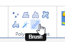
Don’t you hate it? You just spent 2 minutes painstakingly delineating a tissue feature (perhaps using the compound polygon), only to find out that you missed a couple of features.
That’s where the Brush comes in handy. You can use it on pretty much all 2D-annotations (i.e. those that have an area measurements).
The brush and the wand tool are next to each other in the ribbon, because they can actually nicely complement each other: a coarse annotation can be made with the wand, followed by a finetuning around the edges with the brush tool.
What more do you want?
PMA.studio offers advanced annotation tools, specifically designed for the whole slide image data.
We’re not saying we wrote the ultimate set of annotation tools here, but we think we’ve got the basics covered that should help you get pretty far already.
Don’t agree with how we implemented our tools? Need something else? Have an idea for something completely different? Do continue the conversation. We can only get better if you let us know what you’re looking for.
Audit trailing
Our PMA.core tile server is all about providing connectivity, and we talk a lot about how great we are in terms of:
- Supporting more WSI file formats than anybody else
- Supporting more storage media than anybody else
- Being able to integrate different annotations from environments like ImageJ or QuPath
- Being able to bring together a great variety of metadata
What we don’t boast about too often though are our audit trailing capabilities. It’s sort of our secret sauce really, that overlays everything that takes place within the PMA.core environment (and by extension really almost all of our other products, too).
The need for monitoring
Yes, we know that monitoring conjures all sorts of “Big Brother is watching you” memes, but there are a number of good reasons to provide this kind of service, too:
- When enrolling new users, you want to keep an eye out for them that they can do things as they are intended. Some of us are introverts, and some pre-emptive corrections (if needed) may actually be appreciated.
- Too many audit events may be a clue that there’s a security breach in your system, requiring other actions to be initiated.
- It’s a general sanity check for hard working staff that can now at the end of the day make sure that they indeed looked at everything they needed to, and that it was recorded as such.
- During an audit, or when an outlier event takes place, an audit trail can provide supportive evidence that indeed things did take place as intended.
- As a professor, you assign homework cases to your students. Did the student really go look at the assignment?
- In some cases, the features of an audit trail can be prescribed in the form of legal obligations (depending on your jurisdiction). One such example are the FDA’s 21CFR.11 guidelines.
An audit trail need not be a mystery, either. In essence, it means that for each change in any data point, you keep track of:
- Who did it
- When it happened
- Where it happened
- Why it happened
Correspondingly, if there’s no audit trail record of an operation, it didn’t happen.
Creating content
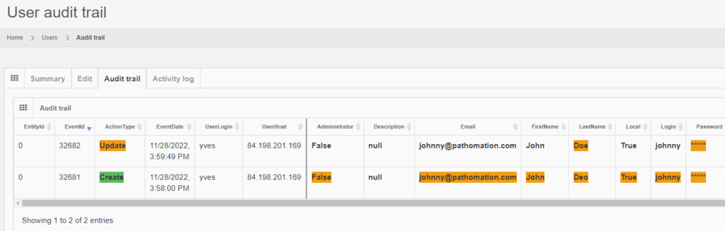
Let’s see how that is implemented in PMA.core. Let’s create a new user:
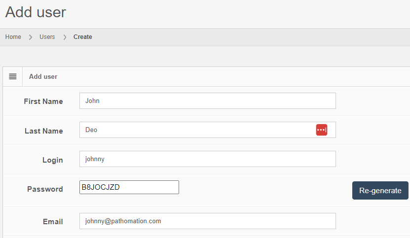
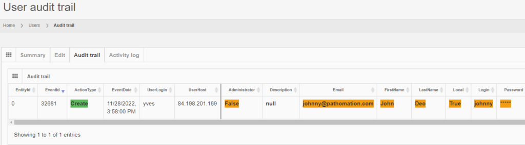
After you create the user, the “Audit trail” tab immediately becomes visible. When you click on it, you see that new data was entered.
The same audit principle applies to other information types across PMA.core. For convenience, we sometimes combine different entities in a single report. An example is a root-directory: A root-directory always consists of a symbolic name (the root-directory itself), and one or more mounting points. You can’t have one without the other. So the audit trail for both is combined and shown as follows:
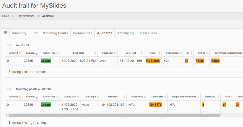
Note that sensitive and private information like someone’s password is still obscured, even at this level.
Editing content
Let’s make some changes to the user’s record:

The audit trail tab shows the changes:
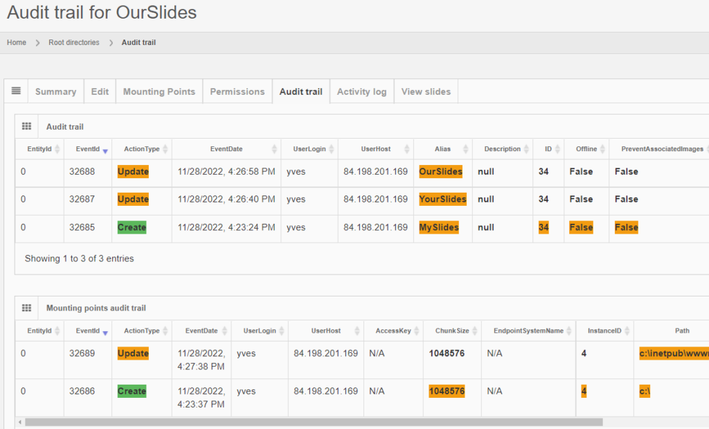
And the same principle applies to all entities, like the aforementioned root-directories. Note that multiple subsequent edits are shown as separate records:
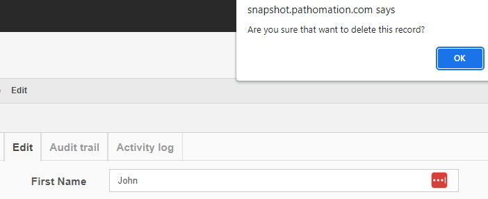
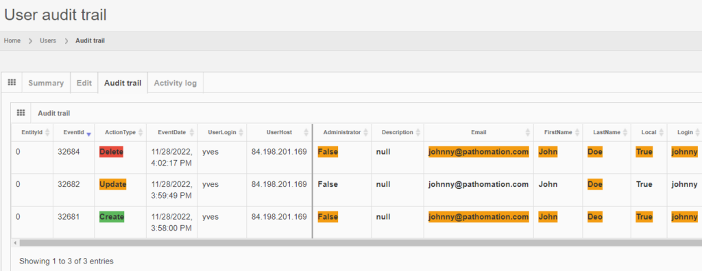
Deleting content
Getting rid of content is probably where the audit trail comes in the most useful.
After deleting a record, you can search for it, and the fact that no results are returned proves that as far as PMA.core is concerned, the record is indeed deleted.
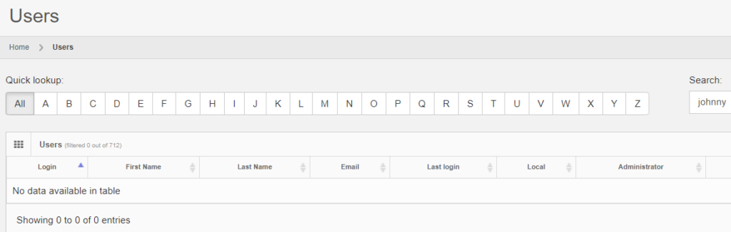
It is possible to transiently see the operation in retrospect, by typing in the direct URL to the entity’s original audit trail:

The red color is used to indicate that something final happened here:
However, when logging out of PMA.core, and logging back it, it’s harder to retrieve the data, as you need to remember to entity’s original identifier, and even if you do, it may be taken over by a new entity.
We’ll show you in a minute how to get access to deleted data in a more reliable and predictable way.
Why would you want to keep track of deleted data? Do you care to find out whether the student did his homework last semester? Probably not, but at least in the context of clinical trials, as well as hospital operations, this makes sense, because:
- Clinical trials can run for many years. For rare diseases, the phase I clinical trial can particularly stretch on for a long time. People switch jobs and roles in between, and when final approval of the drug approaches, it’s important to still have a track record of who was involved
- Regulatory at the country level often require patient data to be kept for dozens of years. Just as important as it is to keep the patient-data, are the meta-data describing the actions performed with the patient records.
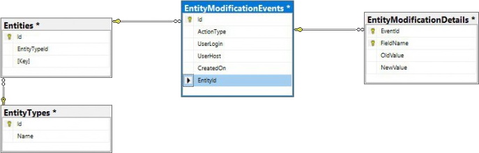
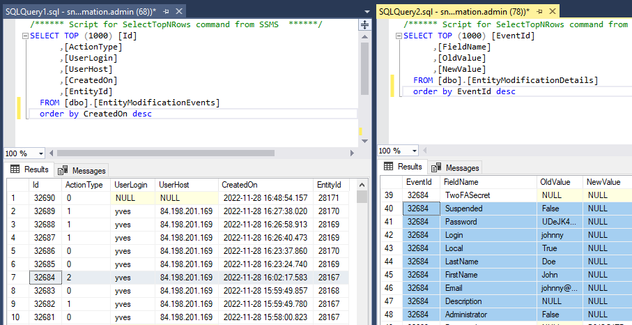
Back-end database
PMA.core only offers audit trail views for the most commonly referenced data types. Whether you can consult the data through the PMA.core end-user interface or not; all operations on any data entities in PMA.core eventually are tracked through a single table structure, which is defined in our wiki:
This means that even if there is no visual interface within PMA.core, or you can’t remember the original URL to the entity’s audit trail, there’s always the possibility to go dig into the audit trail in the back-end:
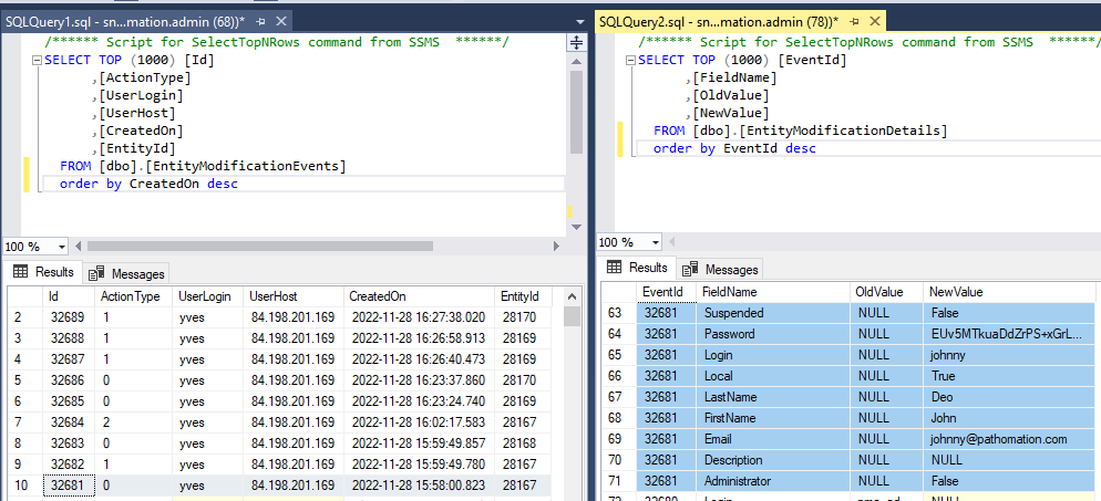
The above shows how the data from our first user record creation is represented. Below is what the update looks like:

And finally, the delete event:
Scaling and resource allocation
All this extra data means extra storage of course. Microsoft SQL Server can definitely handle a lot of records, but there are still situations where extra care is warranted.
When a lot of data passes through the system transiently, it’s possible for the logfiles (tables) to grow quicker than the rest of the database. Consider that also annotations and meta-data (form data) is audit-trailed.
In order to give some guidance as to how much data there actually is, as well as when it was generated, the installation check view gives high-level statistics on this:
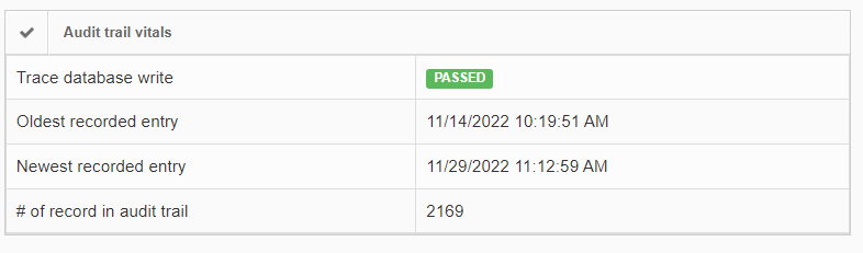
If the number of records in the audit trail increases rapidly, you should be able to explain why this is (many users, lots of annotation activities taking place, lifetime of the total installation…). It’s important also at that point to go through our latest recommendations on SQL Server compliance.
In closing
In an earlier article, we talked about the differences between adapting an open-source strategy versus a commercial platform like our own.
This article adds more substance to this discussion: to be truly prepared for enterprise-level deployment of digital pathology, it’s important to know who’s doing what with your system. It’s important to be able to prove that to the necessary stakeholders, including governments and regulatory agencies.
Pathomation’s PMA.core tile server then has all the necessary infrastructure to get you started off the right foot.