Do you DICOM?

Standardization efforts in digital pathology

DICOM has been working on a standard description of digital pathology (DP) imaging data has been underway for a few years now. Digital pathology and whole slide imaging (WSI) is the focus of DICOM workgroup 26. A summary of its efforts can be found in David Clunie‘s paper in the Journal of Pathology informatics at https://www.ncbi.nlm.nih.gov/pmc/articles/PMC6236926/

In 2014, we published our own conference paper on the effort (during the 12th European Conference on Digital Pathology in Paris, France) . The abstract is available through the Researchgate website; the full presentation from the ECP Paris conference is available through https://www.slideshare.net/YvesSucaet/digital-pathology-information-web-services-dpiws-convergence-in-digital-pathology-data-sharing

The focus of this blog is on imaging. To be complete, readers interested in digital pathology standardization efforts, should also have a look at the IHE PaLM initiative. Additional resources can also be found on slide 45 of our SlideShare publication.

Pathomation supports DICOM

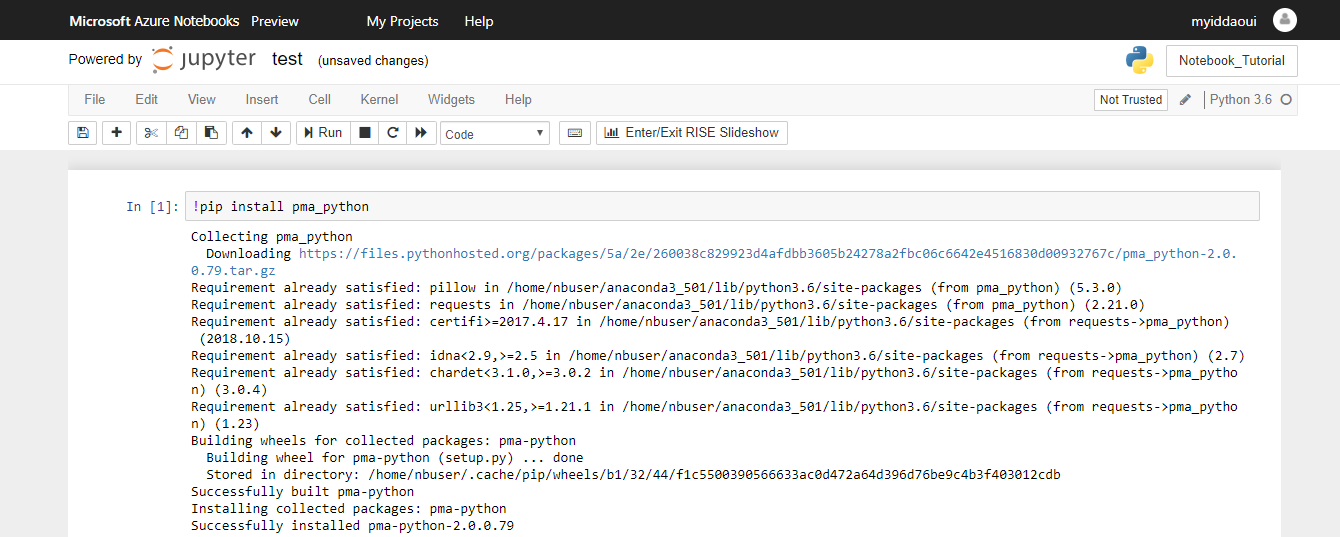
At Pathomation, we’ve been supporting DICOM supplement 145 file format extension (PDF available here) for a while now. We recently added our own “dicomizer” tool to our free PMA.start software. This is a command-line tool (CLI) that allows for the conversion of any WSI file format into a into a DICOM VL (Visible Light) Whole Slide Image IOD (Information Object Definition).

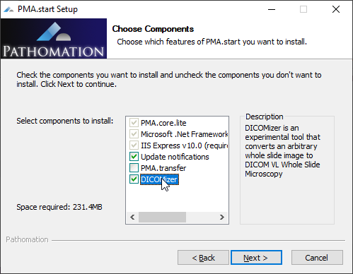
The Pathomation dicomizer is currently available on Windows only (other platforms pending) and can be installed as part of the regular setup process.

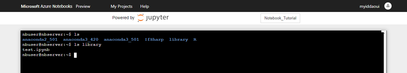
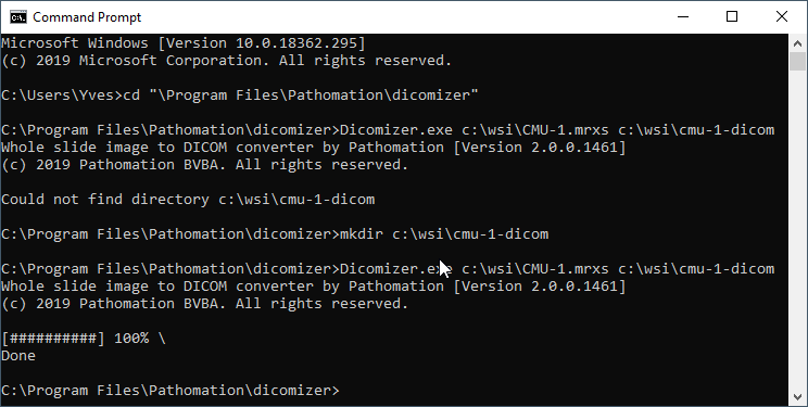
After installation, you have to navigate to the folder in which you installed the tool (typically c:\program files\pathomation\dicomizer) , and then you can invoke the tool through the command-line, like this:

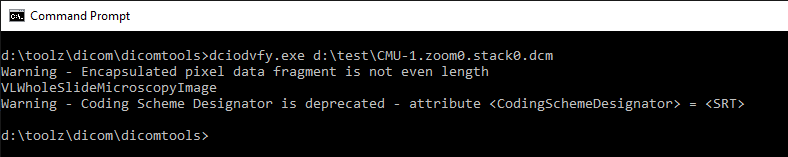
Running the validation tool from David Clunie on our generated DICOM slides results in the following:

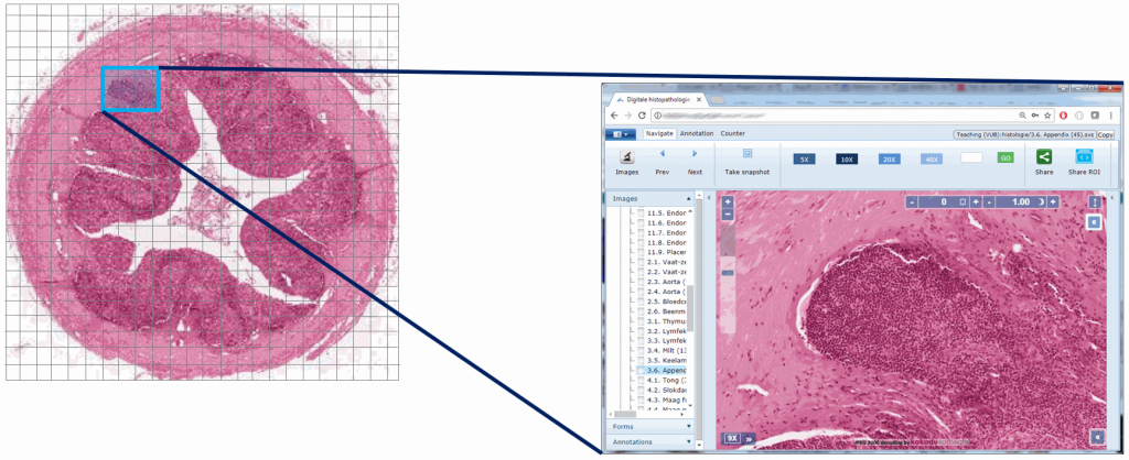
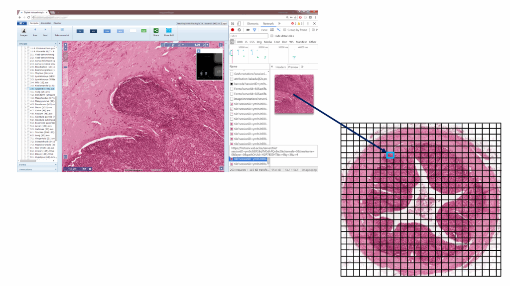
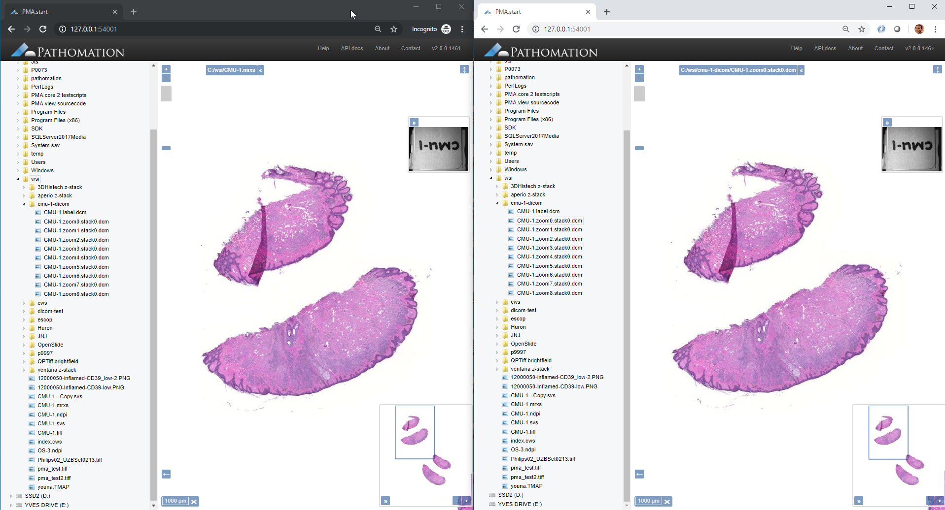
We can also visualize the slides side by side in two browser windows, empirically “proving” that the DICOM output is equivalent to the original slide:

So there you have it. DICOM has been involved in the digital pathology standardization process for a while now. For those interested to support it, you can now use Pathomation’s free dicomizer tool to get hands-on experience.

August 8, 2019March 1, 2023

PHP SDK & Packagist, making your life easier!

Over the past few years, dependency management tools have become a key component to successfully building high-level applications.

The number of third party libraries (with all the dependencies involved) has just insanely grown during the last few years – and expected to grow even more in the upcoming years – that managing the packages, the versions and the dependencies can become a serious nightmare for both developers and project managers. Dependency management tools therefore provide solutions to relieve them of the hassle of keeping dependencies up to date and organized so they can focus on their main mission, building awesome applications.

To make libraries easily shareable online and available for downloads, submissions, updates, bug reporting…Dependency management tools rely naturally on central repositories (we can name Maven central repository for Java, PyPI for python…and the list goes on).

As introduced in our previous posts, our Java SDK is already available on Maven, our Python SDK is also available on PyPI, so the next move logically is to add the PHP SDK to a central repository for PHP to make it easily available for the public…but what do we have for PHP?

For PHP, the dependency management tool to go for is composer, as pointed out earlier, it relies – like other dependency management tools – on its own central repository Packagist.

Installing Composer

In the same logic as most dependency management tools , Composer is available via command line interface which offers indeed way more powerful possibilities than a GUI.
To be able to execute Composer commands, you need to have it installed first on your computer, for more information you can refer to install composer.

Once composer is successfully installed, you can check if your environment is well set up via the following command :

Your first sample code

Next step is to create a sample code to call method getVersionInfo() from Class Core on pma-php (once obviously installed via composer).

To install pma-php via composer in a PHP project, you simply issue the following command in the project folder :

As you could already notice, we didn’t specify any version to install for composer, so it installed automatically the latest release (v2.0.0.40).

Targeting a specified release is straightforward via this command :

For the list of available releases for pma-php library, you can refer to its official Packagist page

Once the library pma-php is successfully installed on a project folder, the following files/folders are created :

Next step is to create a PHP file to call method getVersionInfo() of Class Core on pma-php :


<?php

require_once 'vendor/autoload.php';
use Pathomation\PmaPhp\Core;

echo Core::getVersionInfo();

Running this script returns value “2.0.0.1346”, which is the version of PMA.start installed on my own computer.

That’s all it takes! easy, isn’t it?

August 8, 2019March 1, 2023

Run & share your Python code online with Jupyter notebooks

If you’ve had a look on previous posts on our Python SDK, you have a already a pretty good idea about scripts you can run against PMA.start (or PMA.core) for retrieving image data, Slide visualization…

Most of the times running code locally is all what’s needed, however there are situations where being able to run it online and share it with collaborators (students, colleagues…) on the other side of the globe can come very handy and offer a richer and more interactive experience.
There are couple of free/paid services to run & share Python code online, our focus in this tutorial will be on Azure notebooks powered by Jupyter.

What are Azure notebooks & Jupyter?

As stated on the official documentation, Azure Notebooks is a free service for anyone to develop and run code in their browser using Jupyter. Jupyter is an open source project that enables combing markdown prose, executable code, and graphics onto a single canvas.

Azure Notebooks currently supports Python 2, Python 3, R and F# and their popular packages (e.g for Python the Anaconda distro is preinstalled), but our focus for the moment will be on Python 3 since it’s the minimum required version for the Python SDK

Your first Azure notebooks project

To create your first Azure notebooks project, navigate to the home page
click on Try it now then login (any Microsoft, Gmail,…. email address).

Once successfully logged in, navigate to section My Projects

Click on button New Project :

Introduce a Project name and and ID then click on Create (It’s worth mentioning that you have to set the project as Public if you wish to be able to share your notebooks with other users)

Click on the newly created project :

Notebooks are organized by projects, this makes it very efficient to create separate projects depending on scripts, target hosts and target audience to share notebooks with.

To create a new notebook, click on menu + then select Notebook. Add a name for the notebook and select your Python 3 version (either 3.5 or 3.6 as both compatible with the Python SDK)

Notebooks are organized into cells, each cell can contain one or multiple python scripts to execute.

First cell should always be the following one as it’s required to install first pma_python packages on the running server before being able to interact with the Python SDK.

From there on you can add as many cells as you wish to interact with the Python SDK via scripts we introduced on previous posts or ones you create yourself.

Once your notebook modified and saved, you can easily share the created project with other users via share button on My projects page.

The terminal

In addition to its intuitive and easy-to-use interface, Azure notebooks do provide provides access to a complete terminal running on the server. To access the terminal first click on the Jupyter icon in the upper left hand corner of your notebook server. Then click on the New button on the upper right hand side of the notebook list. Finally click Terminal.

Your newly created notebook is accessible on the running server and executing shell commands there which can be useful for downloading data, copying files, inspecting processes, or editing files with traditional Unix tools.

August 8, 2019

What whole slide images (WSIs) are made of

Whole Slide Images

If you already know about pyramidical image files, feel free to skip this paragraph. If you don’t, sticks around; it’s important to understand how microscopy data coming out of slide scanners is structured to be able to manipulate it.

It all starts with a physical slide: a physical slide is a thin piece of glass, with the dimensions

When a physical slide is registered in a digital fashion, it is translated into a 2-dimensional pixel matrix. At a 40X magnification, it takes a grid of4 x 4 pixels to represent 1 square micrometer. We can also say that the image has a resolution of 0.25 microns per pixel. This is also expressed as 4 pixels per micron (PPM).

All of this means that in order to present our 5 cm x 2 cm physical specimen from the first part of this tutorial series in a 40X resolution we need (5 * 10 * 1000 * 4) * (2 * 10 * 1000 * 4) = 200k x 80k = 16B pixels

Now clearly that image is way too big to load in memory all at once, and even with advanced compression techniques, the physical sizes of these is roughly around one gigabyte per slide. So what people have thought of is to package the image data as a pyramidal stack.

Pyramid of Cestius as a metaphore for pyramidal stack images. By Francesco Gasparetti from Senigallia, Italy – Piramide Cestia, CC BY 2.0, https://commons.wikimedia.org/w/index.php?curid=2614848

Ok, perhaps not that kind of pyramid…

But you can imagine a very large image being downsampled a number of times until it receives a manageable size. You just keep dividing the number of pixels by two, and eventually you get a single image that still represents the whole slide, but is only maybe 782 x 312 pixels in size. This then becomes the top of your pyramid and we label it as zoomlevel 0.

At zoomlevel 1, we get a 1562 x 624 pixel image etc. It turns out that our original image of 200k x 80k pixels is found at zoomlevel 8. Projected onto our pyramid, we get something like this:

Worked out example (showing the different zoomlevels) of a pyramidal stack for a concrete whole slide image.

So the physical file representing the slide doesn’t just store the high-resolution image, it stored a pyramidal stack with as many zoomlevels as needed to reach the deepest level (or highest resolution). The idea is that depending on the magnification that you want to represent on the screen, you read data from a different zoomlevel.

Tiles

The pyramid stack works great up to certain resolution. But pretty quick we get into trouble and the images become too big once again to be shown in one pass. And of course, that is eventually what we want to do: Look at the images in their highest possible detail.

In order to work around this problem, the concept of tiles is introduced. The idea is that at each zoomlevel, a grid overlays the image data, arbitrarily breaking the image up in tiles. This leads to a representation like this:

Now, for any area of the slide that we want to display at any given time to the end-user, we can determine the optimal zoomlevel to select from, as well a select number of tiles that are sufficient to show the desired “field of view”, rather than asking the user to wait to download the entire (potentially huge!) image. This goes as follows:

Or, put the other way around (from the browser’s point of view):

So there you have it: whole slide images are nothing but tiled pyramid-shaped stacks of image data.