Representation
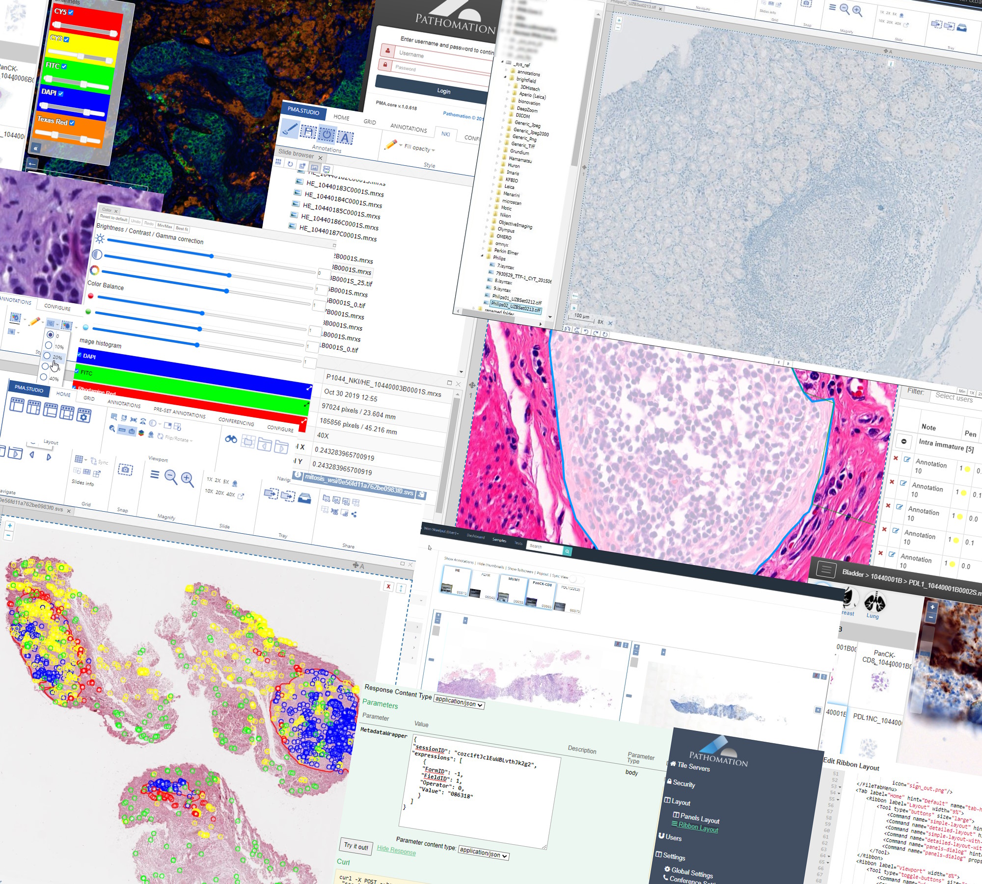
PMA.start is a free desktop viewer for whole slide images. In our previous post, we introduced you to pma_python, a novel package that serves as a wrapper-library and helps interface with PMA.start’s back-end API.
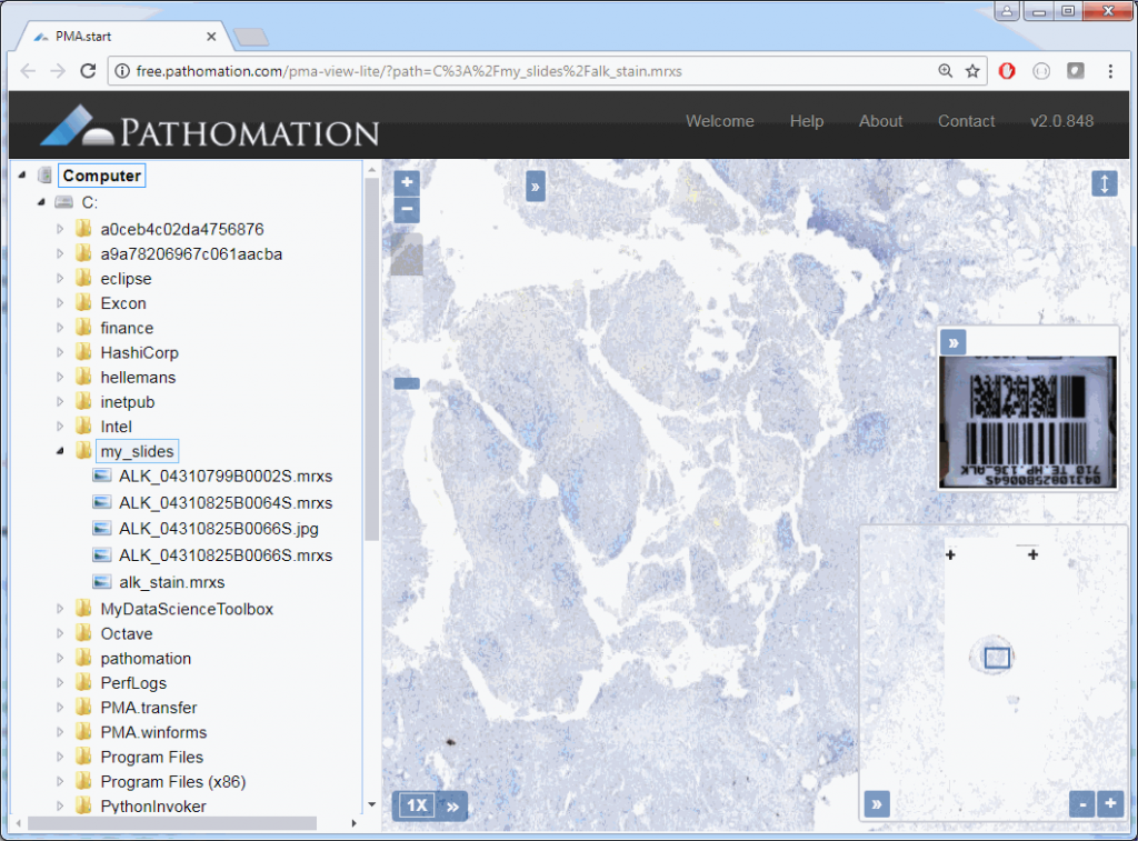
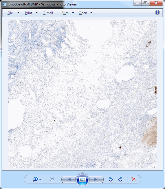
The images PMA.start typically deals with are called whole slide images, so how about we show some pixels? As it turns out, this is really easy. Just invoke the show_slide() call. Assuming you have a slide at c:\my_slides\alk_stain.mrxs, we get:
from pma_python import core
slide =  "C:/my_slides/alk_stain.mrxs"
core.show_slide (slide)
The result depends on whether you’re using PMA.start or a full version of PMA.core. If you’re using PMA.start, you’re taken to the desktop viewer:
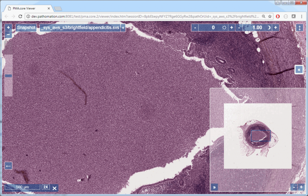
If you’re using PMA.core, you’re presented with an interface with less frills: the webbrowser is still involved, but nothing more than scaffolding code around a PMA.UI.View.Viewport is offered (which actually allows for more powerful applications):
Associated images
But there’s more to these images; if you only wanted to view a slide, you wouldn’t bother with Python in the first place. So let’s see what else we can get out of these?
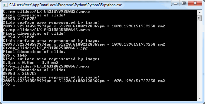
Assuming you have a slide at c:\my_slides\alk_stain.mrxs, you can execute the following code to obtain a thumbnail image representing the whole slide:
from pma_python import pma
slide = "C:/my_slides/alk_stain.mrxs"
thumb = core.get_thumbnail_image(slide)
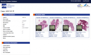
thumb.show()But this thumbnail presentation alone doesn’t give you the whole picture. You should know that a physical glass slide usually consists of two parts: the biggest part of the slide contains the specimen of interest and is represented by the thumbnail image. However, near the end, a label is usually pasted on with information about the slide: the stain used, the tissue type, perhaps even the name of the physician. More recently, oftentimes the label has a barcode printed on it, for easy and automated identification of a slide. The label is therefore sometimes also referred to as “barcode”. Because the two terms are used so interchangeably, we decided to support them in both forms, too. This makes it easier to write code that not only syntactically makes sense, but also applies semantically in your work-environment.
A systematic representation of a physical glass slide can then be given as follows:

The pma_python library then has three methods to obtain slide representations, two of which are aliases of one another:
core.get_thumbnail_image() returns the thumbnail image
core.get_label_image() returns the label image
core.get_barcode_image() is an alias for get_label_image
All of the above methods return PIL Image-objects. It actually took some discussion to figure out how to package the data. Since the SDK wraps around an HTTP-based API, we settled on representing pixels through Pillows. Pillows is the successor to the Python Image Library (PIL). The package should be installed for you automatically when you obtained pma_python.
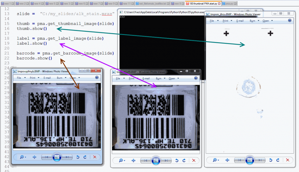
The following code shows all three representations of a slide side by side:
from pma_python import core
slide =  "C:/my_slides/alk_stain.mrxs"
thumb = core.get_thumbnail_image(slide)
thumb.show()
label = core.get_label_image(slide)
label.show()
barcode = core.get_barcode_image(slide)
barcode.show()
The output is as follows:
Note that not all WSI files have label / barcode information in them. In order to determine what kind of associated images there are, you can inspect a SlideInfo dictionary first to see what’s available:
info = core.get_slide_info(slide)
print(info["AssociatedImageTypes"])
AssociatedImageTypes may refer to more than thumbnail or barcode images, depending on the underlying file format. The most common use of this function is to determine whether a barcode is included or not.
You could write your own function to determine whether your slide has a barcode image:
def slide_has_barcode(slide):
    info = core.get_slide_info(slide)
    return "Barcode" in info["AssociatedImageTypes"]
Tiles in PMA.start
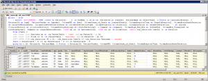
We can access individual tiles within the tiled stack using PMA.start, but before we do that we should first look some more at a slide’s metadata.
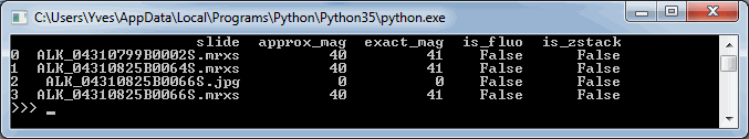
We can start by making a table of all zoomlevels the tiles per zoomlevel, along with the magnification represented at each zoomlevel:
from pma_python import pma
import pandas as pd

level_infos = []
slide = "C:/my_slides/alk_stain.mrxs"
levels = core.get_zoomlevels_list(slide)
for lvl in levels:
    res_x, res_y = core.get_pixel_dimensions(slide, zoomlevel = lvl)
    tiles_xyz = core.get_number_of_tiles(slide, zoomlevel = lvl)
    dict = {
        "res_x": round(res_x),
        "res_y": round(res_y),
        "tiles_x": tiles_xyz[0],
        "tiles_y": tiles_xyz[1],
        "approx_mag": core.get_magnification(slide, exact = False, zoomlevel = lvl),
        "exact_mag": core.get_magnification(slide, exact = True, zoomlevel = lvl)
     }
     level_infos.append(dict)

df_levels = pd.DataFrame(level_infos, columns=["res_x", "res_y", "tiles_x", "tiles_y", "approx_mag", "exact_mag"])
print(slide)
print(df_levels)
The result for our alk_stain.mrxs slide looks as follows:
Now that we have an idea of the number of zoomlevels to expect and how many tiles there are at each zoomlevel, we can request an individual tile easily. Let’s say that we wanted to request the middle tile at the middle zoomlevel:
slide = "C:/my_slides/alk_stain.mrxs"
levels = core.get_zoomlevels_list(slide)
lvl = levels[round(len(levels) / 2)]
tiles_xyz = core.get_number_of_tiles(slide, zoomlevel = lvl)
x = round(tiles_xyz[0] / 2)
y = round(tiles_xyz[1] / 2)
tile = core.get_tile(slide, x = x, y = y, zoomlevel = lvl)
tile.show()
This should pop up a single tile:
.Ok, perhaps not that impressive.
In practice, you’ll typically want to loop over all tiles in a particular zoomlevel. The following code will show all tiles at zoomlevel 1 (increase to max_zoomlevel at your own peril):
tile_sz = core.get_number_of_tiles(slide, zoomlevel = 1) # zoomlevel 1
for xTile in range(0, tile_sz[0]):
    for yTile in range(0, tile_sz[1]):
        tile = core.get_tile(slide, x = xTile, y = yTile, zoomlevel = 1)
        tile.show()
The advantage of this approach is that you have control over the direction in which tiles are processed. You can also process row by row and perhaps print a status update after each row is processed.
However, if all you care about is to process all rows left to right, top to bottom, you can opt for a more condensed approach:
for tile in core.get_tiles(slide, toX = tile_sz[0], toY = tile_sz[1], zoomlevel = 4):
    data = numpy.array(tile)
The body of the for-loop now processes all tiles at zoomlevel 4 one by one and converts them into a numpy array, ready for image processing to occur, e.g. through opencv. But that will have to wait for another post.