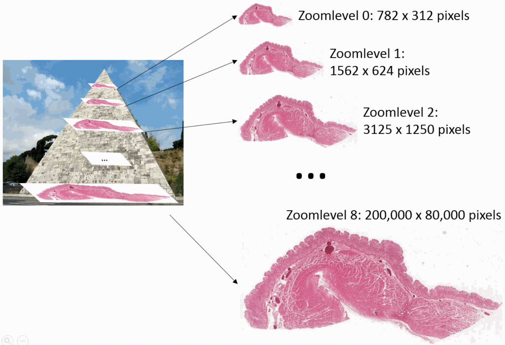
Educational needs and virtual microscopy

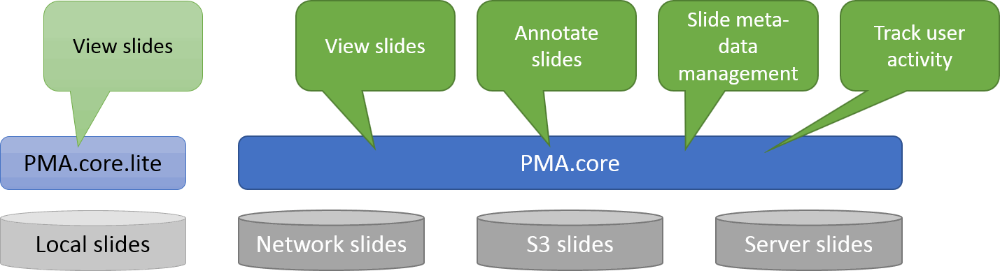
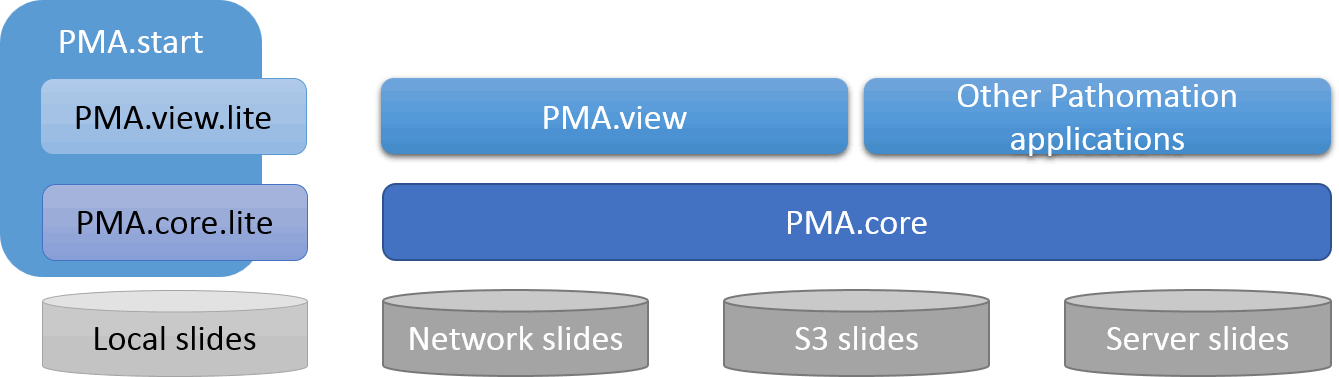
Pathomation’s software platform includes software for a number of digital pathology application.

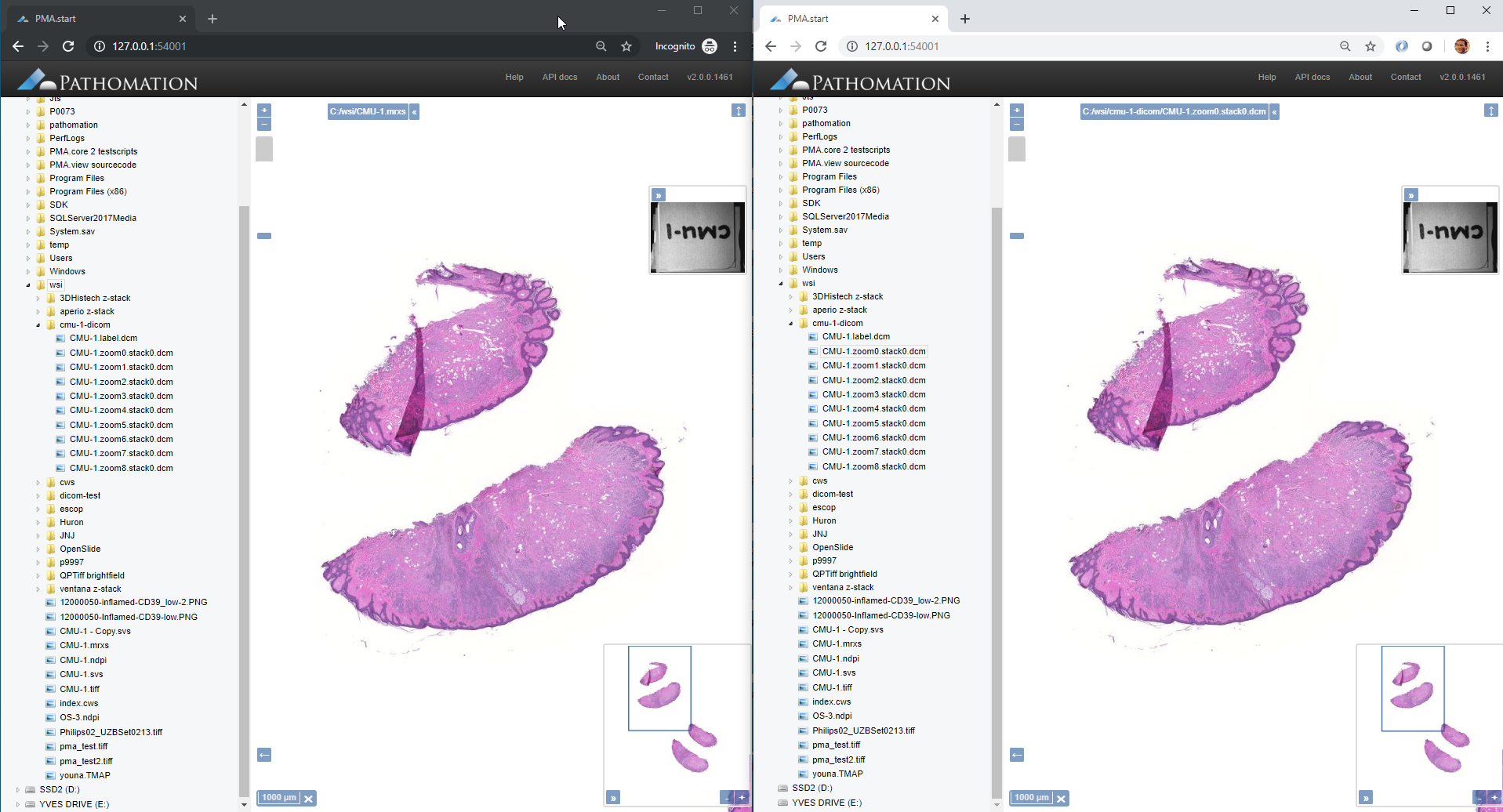
At the most basic end of the spectrum we offer PMA.start for local viewing and research purposes. Even with PMA.start, you get full access to our front-end Javascript-based visualization framework, and back-end automation API (more on those in a separate blogpost).

• 

At the opposite end of the spectrum, we offer a sophisticated training software package called PMA.control. Consider this:

• Current slide-based approaches to microscopy teaching face the logistical challenge of transporting people, slides and training material.
• The size, location and number of instructional sessions is limited (in time, place, and size)
• Concurrent training on the same material is not possible. One microscope can offer one unique slide. Musical chair… erh… microscopes, anyone?

We identified a need has evolved to train students and professionals alike to accurately evaluate tissue material with a broad range of (assay-specific) algorithms. Systematically organizing training materials and bringing training participants together in a virtual settings, is what it’s all about.

Projects

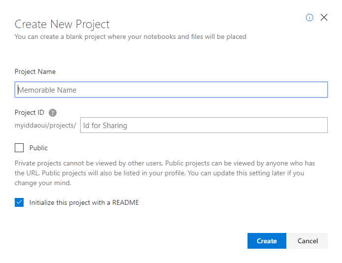
You start in PMA.control by setting up a project. A project describes what it is that you want to organize instructional material around. A project can represent a course at a university, or a drug for a pharma company. A project can delineate a geographical territory. It’s totally up to you.

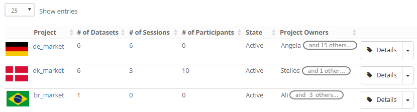
Projects have various properties. Apart from their name, you can identify them with an icon. This is convenient as your list of project becomes larger and more people become involved in your project. Speaking of involved people: you can identify one or more project managers. This is particularly useful for larger organizations, where one person is seldom available all the time, but it’s relatively easy to find a replacement in case of absence.

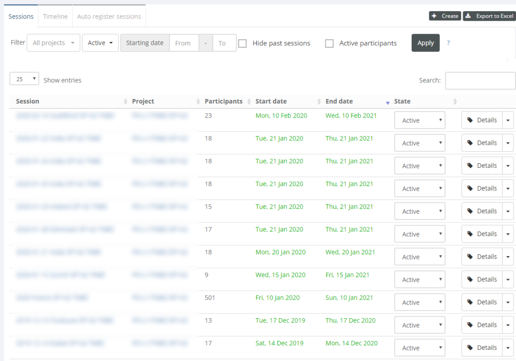
Training sessions

A project consists of training sessions. Again, what these mean semantically is completely up to you and your imagination:

1. One client of ours uses PMA.control to organize weekly seminars in various places across the globe. Each seminar/country combination translates into its own training session in PMA.control, with specific start- and end-dates
2. One medical school uses PMA.control to train residents. A training session can refer to the class coming in on a particular week, but it can also be linked to small research projects that students participate in.
3. Another client integrates PMA.control into a web-portal, so all training sessions by definitions are open ended. The client has a drug portfolio, so rather than have them be restricted in time, training sessions refer to various indications for different drugs.

Safe to say that training sessions can be exploited for diverse applications.

Case collections

All right, we have projects and training sessions… When do we put digital slide content in them? This is where case collections come in.

The idea is that you organize your training sessions in different parts. During a three-day seminar, you could have one day dedicated to guided lectures (that’s a case collection with its own slides). On day two, you allow people to evaluate themselves through some hands-on exercises (on a second case collection, which holds different slides than the first one). On day three, it’s crunch time, and attendees take an actual test to see how well they absorbed the material (on yet another third case collection with once again unique slides).

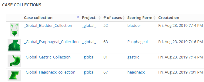
A case collection is coupled to a project, but is independent from any training sessions, so you can re-use them throughout the curriculum that you’re building. Think about it; otherwise if you organized the same training session repeatedly, you would continuously have to re-define the case collections, too!

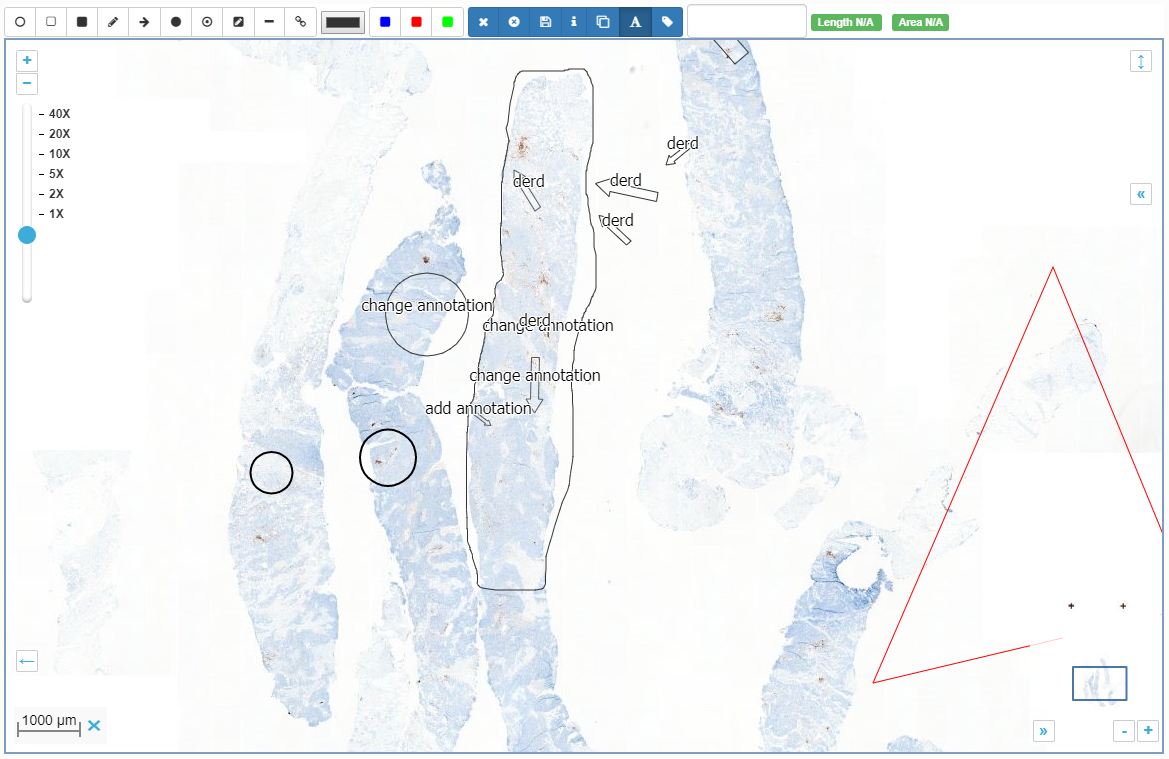
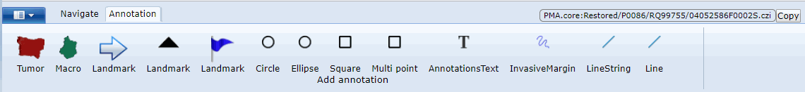
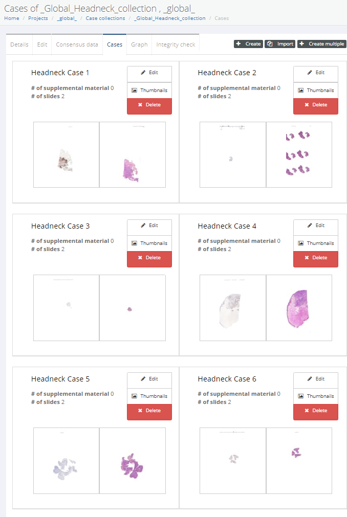
A case collection consists of cases, which in turn consist of slides. You can choose to construct a case such that it pre-focuses on a particular region of interest (ROI) within a slide. You can also add various meta-data at case-level as well as slide-level. Not unimportantly: you can configure the initial rotation angle for each slide in the case. This is particularly relevant if your case consists of serial sections that may not be all in the exact same orientation.

Interaction modes

Remember the three-day seminar we just mentioned? And you also remember that we called the software “PMA.control”, right?

Ok.

The name PMA.control refers to the fact that the owner of the software is in total control of what participants within a session at any given time.

Consider the following situations during our three-day seminar:

• On the first day, the instructor wants his pupils to stay nicely in the kiddie pool. They should give their undivided attention only to the material intended for the first day.
• However, this one person in the afternoon of the first day is taking the seminar for the second time. She asks if she can skip ahead already to the content from day two.
• On the second day, people are learning and experimenting with a different dataset. Do they understand the material well enough to pass the test on the last day? Clearly the material from day three must not be visible to anybody yet.
• On day three, it’s crunch time. The actual test material is now released. Depending on the intention of the instructor, earlier discussed material can now even be closed off.

For all these conditions, PMA.control offers interaction modes. An interaction mode controls if and how a case collection presents itself to the end-user.

Training sessions consist of multiple case collections and multiple users participate in a training session. At any given time, the instructor of a session can specify whether a particular case collection within the session is accessible to a specific user and how.

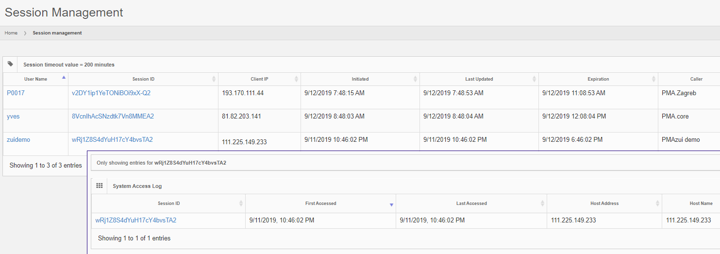
When signing into PMA.control, the instructor sees a grid with users and case collections. This grid can be used to control what user interacts with what case collection.

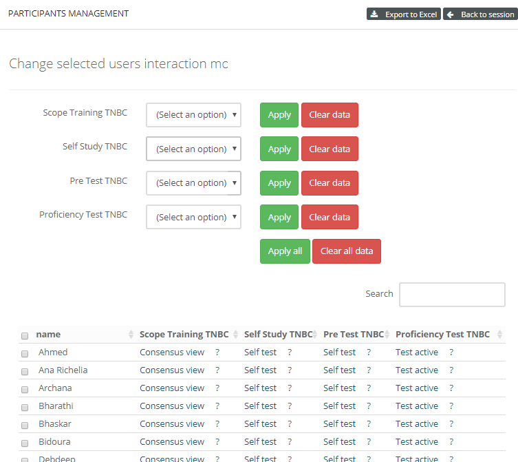
PMA.control ships with a number of default interaction modes, but these can be customized via a matrix interface where one stipulates what properties are associated with each.

Let’s see how interaction modes come into play during our three-day seminar:

• Before leaving for the seminar, the instructor applies the interaction mode “locked” to all case collections for all participants.
• On the morning of the first day, the instructor walks in the seminar room an hour early an sets the interaction mode of the first case collection to “browse” for everybody to see. That was easy! He goes to the hotel bar to grab a nice cup of coffee.
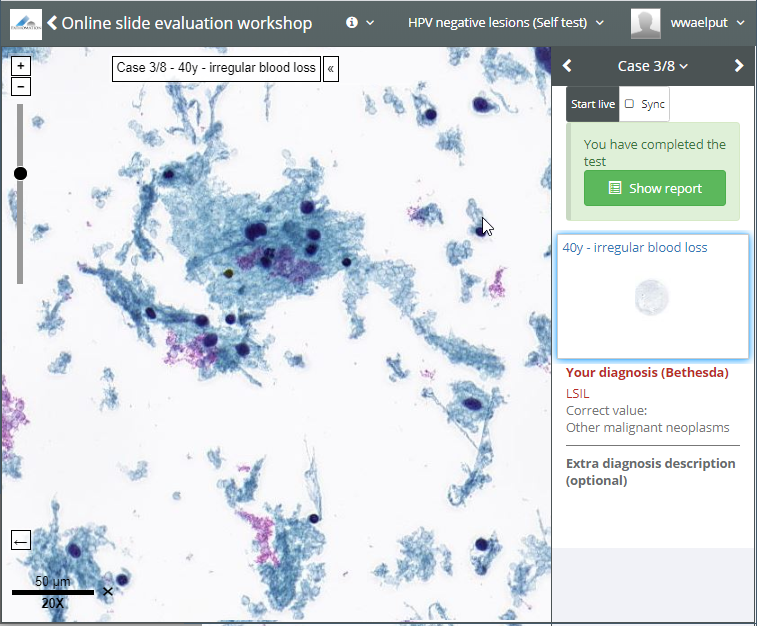
• In the afternoon of the first day, an attendee asks about being allowed to skip ahead with the material a bit. The instructor asks if any other people are in the same situation. For those, he sets the interaction mode for the second case collection to “self-test”. Users can interactively fill out a pre-determined scoring form that goes with each case, and they can see each other’s results to discuss their findings amongst themselves.
• On the second day, the second case collection is unlocked for everybody. Everybody now sees the second case collection in self-test mode. The first case collection remains in “browse” mode, so participants can use these as reference material. The third case collection remains off limits today.
• On the morning of the third day, the first thing the instructor does is reset the first and second case collection in the training session to “locked”. Rien ne va plus. The third and last case collection is switched to “test”, and students can take their final assessment. Users can interactively fill out a pre-determined scoring form that goes with each case, but they can’t see each other’s data anymore.

It’s possible for an instructor to be an instructor for one session, but only a “regular” participant in another. This is especially useful in medical schools where different specialists consult with and train each other on various subject matters on a continuous basis.

Conclusion

PMA.control allows you to assemble whole-slide images, scoring forms, consensus scores and scoring manuals into digital training modules. Full service, no-hassle, management of the software is offered through the PathoTrainer service, which is organized through Pathomation’s parent company CellCarta .

If you’re interested in higher education teaching of histology or pathology, make sure to also have a look at Pathomation’s education landing page. For pharma and CRO application, we have a separate landing page.

Blurred or focused?

In an earlier post, we offered some ideas on how to detect tissue in a scanned slide.

The next step people often want to take is to examine how the sharpness of the tissue is distributed throughout the slide. No scanner catches all, and you will see blurry areas in pretty much all your scans.

It then helps to be able to differentiate the tiles that have poor focus from the tiles that are sharp. As it turns out, we already approached a likewise problem when we were determining the sharpest tiles within z-stacked slides.

For this particular exercise (focus variation within a single plane) Sied Kebir in Germany was kind enough to provide us with relevant sample data for this one.

And here are two relevant extracted tiles to illustrate the problem.

Sied is looking for a method to systematically map the blurry tiles vs the crisp ones.

Blur detection with OpenCV

A good introduction on blur detection with the OpenCV library is offered by pysource in the following video tutorial:

Let’s see what that gives when we apply it to Sied’s sample images:

Great! The numbers are not as far apart as in pysource’s video, but that makes sense: even in focused tissue we’ll find many more gradients and sloping color ranges than in the average picture of person sitting a room, which contains distinctive features like outlined walls and facial contours.

Pysource suggests converting your original images to grayscale. Does it make a difference? In our experiments we find different values (of course), but the trend is the same. Since the retention color of leads to slightly bigger differences, we’re inclined to sticking with the original color images.

If you do want to convert your color tiles to grayscale, here’s a great StackOverflow article about how this works.

Distribution and Exploratory Data Analysis (EDA)

Our next step is to put it all in a loop and systematically examine how sharp or blurry each individual tile actually is. For semantic ease, we create a get_blurriness function:

from pma_python import core
import matplotlib.pyplot as plt
import numpy as np
import scipy.stats
import sys

def is_tissue(tile):
    pixels = np.array(tile).flatten()
    mean_threahold = np.mean(pixels) < 192   # 75th percentile
    std_threshold = np.std(pixels) < 75
    return mean_threahold == True and std_threshold == True

def is_whitespace(tile):
    return not is_tissue(tile)

def get_sharpness(img):
    pixels = np.array(img).flatten()
    return cv2.Laplacian(pixels, cv2.CV_64F).var()

slide = "C:/wsi/sied/test.svs"
max_zl = 5 # or set to core.get_max_zoomlevel(slide)
dims = core.get_zoomlevels_dict(slide)[max_zl]

means = []
stds = []
tissue_map = []
sharp_map = []

for x in range(0, dims[0]):
    for y in range(0, dims[1]):
        tile = core.get_tile(slide, x=x, y=y, zoomlevel=max_zl)
        tiss = is_tissue(tile)
        tissue_map.append(tiss)
        if (tiss):
            sharp_map.append(get_sharpness(tile))
        else:
            sharp_map.append(0)
    print(".", end="")
    sys.stdout.flush()
print()

After getting all the result, it is worth examining the histogram of this data.

Ideally, we would like to see a bimodal distribution (sharp vs blurred), but that’s not what we see here. The reason is that unevenness in tissue is actually not distributed unevenly.

Putting it all together

Now that we know what we can expect, it’s just a matter of putting it all together. and use it to construct an image map, in similar fashion as we did for our original tissue detection.

The final result looks like this:

In closing

Sectioning a slide is a continuous operation, and except for folding artifacts, you shouldn’t expect any abrupt changes. Tissue can be expected to gradually fade in and out of focus. And while scanners have gotten better at compensating for uneven tissue thickness, we’re not quite there yet, and automated analysis based on a technique like we’re here proposing can help.

Last but now least, we decided on a new way to organize our sample code. At http://host.pathomation.com/realdata/ you can from now on see all sample data in a single location. For example, the Jupyter notebook that belongs with this entry, is available at http://host.pathomation.com/realdata/jupyter/realdata%20033%20-%20look%20sharp.ipynb

A customer query

As part of our commercial offering, Pathomation offers hosting services for those organization that don’t want to make a long term investment in on-premise server hardware, or whose server farm is incompatible with our system requirements (PMA.core requires a Microsoft Windows stack).

One such customer came to us recently and asked how much space they were consuming on the virtual machine they rented from us.

This was our answer:

And this is how we obtained the answer. We wrote the following script:

In Python:

from pma_python import core
def get_slide_size(session, slideRef):
    info = core.get_slide_info(slideRef, sessionID = session)
    return info["PhysicalSize"]
def get_total_storage(session, path):
    total = 0
    for slide in core.get_slides(path, session, True):
        total = total + get_slide_size(session, slide)
    return total
def map_storage_usage(srv, usr, pwd):
    sess = core.connect(srv, usr, pwd)
    map = {}
    for rd in core.get_root_directories(sess):
        map[rd] = get_total_storage(sess, rd)
    return map

You can also do this in PHP, of course:

<?php
require "lib_pathomation.php"; 	// PMA.php library

use Pathomation\PmaPhp\Core;

function getTotalStorage($sessionID, $dir) {
        $slides = Core::getSlides($dir, $sessionID, $recursive = FALSE);
        $infos = Core::GetSlidesInfo($slides, $sessionID);
        
        echo "Got slides for ".$dir.PHP_EOL;

        $func = function($value) {
            return $value["PhysicalSize"];
        };

        $s = array_sum(array_map($func, $infos));
        return $s;
}

function mapStorageUsage($serverUrl, $username, $password) {
    $sessionID = Core::Connect($serverUrl, $username, $password);
    
    $map = array();
    $rootdirs = Core::getRootDirectories($sessionID);
    foreach ($rootdirs as $rd) {
        $map[$rd] = getTotalStorage($sessionID, $rd);
        
    }
    return $map;
}
?>

Creating a dictionary that contains the number of consumed bytes per root-directory now comes down to using just a single line of code:

In Python:

print(map_storage_usage("http://server/pma.core",
"user", "secret_password"))

And in PHP:

print_r( mapStorageUsage ("http://server/pma.core", "user", "secret_password")); 

Making our code mode robust

Unfortunately, chances are that if you’ve been running your PMA.core tile server for a while, the script comes down crashing miserably. It the “should have could have would have” syndrome of programming. There’s probably a meme for this out there somewhere (in the interest of productivity, we won’t search for it ourselves but let you look for that one). What it comes down to is: mounting points and access permissions chance, and at some point in time in any large enough data repository some files are going to end up corrupt, meaning either the core.get_slides() call is going to go wrong, or the core.get_slide_info() call.

So to make our script a bit more robust, we can add try… catch… exception handling in Python:

def get_slide_size(session, slideRef):
    try:    
        info = core.get_slide_info(slideRef, sessionID = session)
        return info["PhysicalSize"]
    except:
        print("Unable to get slide information from", slideRef)
        return 0

def get_total_storage(session, path):
    total = 0
    try:
        for slide in core.get_slides(path, session, True):
            total = total + get_slide_size(session, slide)
    except:
        print("unable to get data from", path)
    return total

def map_storage_usage(srv, usr, pwd):
    sess = core.connect(srv, usr, pwd)
    map = {}
    for rd in core.get_root_directories(sess):
        map[rd] = get_total_storage(sess, rd)
    return map

As well as in PHP:

<?php
require_once "lib_pathomation.php";

use Pathomation\PmaPhp\Core;

function getTotalStorage($sessionID, $dir) {
    try {
        $slides = Core::getSlides($dir, $sessionID, $recursive = FALSE);
        $infos = Core::GetSlidesInfo($slides, $sessionID);
        
        $func = function($value) {
            return $value["PhysicalSize"];
        };

        $s = array_sum(array_map($func, $infos));
        return $s;
    }
    catch(Exception $e) {
        // echo "unable to get data from ".$dir.PHP_EOL;
    }
}

function mapStorageUsage($serverUrl, $username, $password) {
    $sessionID = Core::Connect($serverUrl, $username, $password);    
    $map = array();
    $rootdirs = Core::getRootDirectories($sessionID);
    foreach ($rootdirs as $rd) {
        $map[$rd] = getTotalStorage($sessionID, $rd);   
    }
    return $map;
}

print_r(mapStorageUsage("http:/server/core/", "user", "secret"));
?>

In Python, you can also add the prettyprint library to clean up the output a bit:

And in PHP, we add a convenient method to make the numbers a bit easier to read:

function human_filesize($bytes, $decimals = 2) {

    $size = array('B','kB','MB','GB','TB','PB','EB','ZB','YB');

    $factor = floor((strlen($bytes) - 1) / 3);

    return sprintf("%.{$decimals}f", $bytes / pow(1024, $factor)) . @$size[$factor];

}

Input for business intelligence (BI)

In this article we showed how you can use automation to let Pathomation’s PMA.core tile server generate an overview report of how much space your slides consume. Depending on your specific folder structure, you can further customize this for breakdowns into sizable data-morsels that fit your particular appetite.

Given the size of the average size of a slide, this kind of information can be vital to your organization: Slides can accumulate fast, and it is important to keep a handle on their growth and space occupation.

Pathomation’s software platform is more than just a slide viewing solution: it can help to generate insights in your storage resource consumption and be used as a veritable planning and evaluation tool before actual investments take place.

A question we get frequently from potential customers is “how do we import our slides into your system (PMA.core)?”. The answer is: we don’t. In contrast with other Image Management Systems (IMS), we opted to not go for a central database. In our opinion, databases only seem like a good idea at first, but inevitable always cause problems down the road.

People also ask us “how easy is it to import our slides?”. The latter phrasing is probably more telltale than the first, as it assumes that is not the case apparently with other systems, i.e., other systems often put you in a situation where it is not easy to register slides. It still puts us in an awkward position, as we then actually have to explain that there is no import process as such. Put the slides where you want them, and that’s it. You’re done. Finito.

Here are some of the reasons why you would want a database overlaying your slides:

• Ease of data association. Form data and overlaying graphical annotation objects can be stored with the slide’s full path reference as a foreign key.
• Ease of search for a specific slide. Running a search query on a table is decidedly faster than parsing a potentially highly hierarchical directory tree structure
• Rapid access to slide metadata. Which is not the same as our first point: data association. Slide metadata is information that is already incorporated into the native file format itself. A database can opt to extract such information periodically and store it internally in a centralized table structure, so that it is more easily extracted in real time when needed.

When taken together, the conclusion is that such databases are nothing more but glorified indexing systems. Such an indexing system invariable turns into a gorilla… An 800 lbs gorilla for that matter… Let’s talk about it:

• An index takes time to build
• An index consumes resources, both during and after construction.
• With a rapidly evolving underlying data structure, the index is at risk of being behind the curve and not reflecting the actual data
• In order to control the index and not constantly having to rebuild it, a guided (underlying) data management approach may be needed
• At some point, in between index builds, and outside the controlled data entry flow, someone is going to do something different to your data
• Incremental index builds to bypass performance bottlenecks are problematic when data is updated

Now there are scenarios where all of the above doesn’t matter, or at least doesn’t matter all that much. Think of a conventional library catalog; does it really matter if your readers can only find out about the newest Dean Koontz book that was purchased a day after it was actually registered in the system? Even with rapidly moving inventory systems: when somebody orders an item that is erroneously no longer available from your webstore… Big whoop. The item is placed on back-order, or the end-user simply cancels the order. It you end up making the majority of your customers mad this way, then the problem is not in your indexing system, but in your supply chain itself. There’s no doubt that for webshops and library catalogs, indexes speed up search, and the pros on average outweigh the cons.

But digital pathology is different. Let’s look at each of the arguments against indexing and see how much weight they carry in a WSI environment:

• An index takes time to build. When are you going to run it? Digital pathology was created so you can have round the clock availability of your WSI data. Around the clock. Across time-zones. Anything that takes time, also takes resources. CPU cycles, memory. So expect performance of your overall system to go down while this happens.
• Resource (storage) consumption during and after construction. So be careful about what you are going to index in terms of storage. Are you going to index slide metadata? Thumbnails? How much data are your practically talking about? How much data are you going to index to begin with? And how much of your indexed data will realistically ever be accessed (more on that subject in a separate post)?
• Rapidly evolving underlying data structure. Assume a new slide is generated once every two minutes, and a quantification algorithm (like HistoQC) takes about a minute to complete per slide. This means you have a new datapoint every minute. And guess which datapoint the physician wants to see now now NOW…
• Guided data management approach. One of the great uses of digital pathology is the sharing of data. You can share your data, but other can also share it with you. So apart from your in-house scanner pipeline; what do you going to do with the external hard disk someone just sent you? Data hierarchies come in all shapes and sizes. Sometimes it’s a patient case; sometimes it’s toxicological before/after results; sometimes it’s a cohort from a drug study. Are you going to setup data import pipelines for all these separate scenarios? Who’s going to manage those?
• Sometimes, somewhere, someone is going to do something different to your data. Because the above pipelines won’t work. No matter how carefully you design them. Sometimes something different is needed. You need to act, and there’s no time for re-design first. The slide gets replaced, and now the index is out-of-date. Or the slide is renamed because of earlier human error, and the index can’t find it anymore. And as is often the case: this isn’t about the scenarios that you can think of; but about the scenarios you can’t.

Safe to say that we think an indexing mechanism for digital pathology and whole slide images is not a good idea. Just don’t do it.

Standardization efforts in digital pathology

DICOM has been working on a standard description of digital pathology (DP) imaging data has been underway for a few years now. Digital pathology and whole slide imaging (WSI) is the focus of DICOM workgroup 26. A summary of its efforts can be found in David Clunie‘s paper in the Journal of Pathology informatics at https://www.ncbi.nlm.nih.gov/pmc/articles/PMC6236926/

In 2014, we published our own conference paper on the effort (during the 12th European Conference on Digital Pathology in Paris, France) . The abstract is available through the Researchgate website; the full presentation from the ECP Paris conference is available through https://www.slideshare.net/YvesSucaet/digital-pathology-information-web-services-dpiws-convergence-in-digital-pathology-data-sharing

The focus of this blog is on imaging. To be complete, readers interested in digital pathology standardization efforts, should also have a look at the IHE PaLM initiative.  Additional resources can also be found on slide 45 of our SlideShare publication.

Pathomation supports DICOM

At Pathomation, we’ve been supporting DICOM supplement 145 file format extension (PDF available here) for a while now. We recently added our own “dicomizer” tool to our free PMA.start software. This is a command-line tool (CLI) that allows for the conversion of any WSI file format into a into a DICOM VL (Visible Light) Whole Slide Image IOD (Information Object Definition).

The Pathomation dicomizer is currently available on Windows only (other platforms pending) and can be installed as part of the regular setup process.

After installation, you have to navigate to the folder in which you installed the tool (typically c:\program files\pathomation\dicomizer) , and then you can invoke the tool through the command-line, like this:

Running the validation tool from David Clunie on our generated DICOM slides results in the following:

We can also visualize the slides side by side in two browser windows, empirically “proving” that the DICOM output is equivalent to the original slide:

So there you have it. DICOM has been involved in the digital pathology standardization process for a while now. For those interested to support it, you can now use Pathomation’s free dicomizer tool to get hands-on experience.

 

 

 

 

 

Whole Slide Images

If you already know about pyramidical image files, feel free to skip this paragraph. If you don’t, sticks around; it’s important to understand how microscopy data coming out of slide scanners is structured to be able to manipulate it.

It all starts with a physical slide: a physical slide is a thin piece of glass, with the dimensions

When a physical slide is registered in a digital fashion, it is translated into a 2-dimensional pixel matrix. At a 40X magnification, it takes a grid of4 x 4 pixels to represent 1 square micrometer. We can also say that the image has a resolution of 0.25 microns per pixel. This is also expressed as 4 pixels per micron (PPM).

All of this means that in order to present our 5 cm x 2 cm physical specimen from the first part of this tutorial series in a 40X resolution we need (5 * 10 * 1000 * 4) * (2 * 10 * 1000 * 4) = 200k x 80k = 16B pixels

Now clearly that image is way too big to load in memory all at once, and even with advanced compression techniques, the physical sizes of these is roughly around one gigabyte per slide. So what people have thought of is to package the image data as a pyramidal stack.

Ok, perhaps not that kind of pyramid…

But you can imagine a very large image being downsampled a number of times until it receives a manageable size. You just keep dividing the number of pixels by two, and eventually you get a single image that still represents the whole slide, but is only maybe 782 x 312 pixels in size. This then becomes the top of your pyramid and we label it as zoomlevel 0.

At zoomlevel 1, we get a 1562 x 624 pixel image etc. It turns out that our original image of 200k x 80k pixels is found at zoomlevel 8. Projected onto our pyramid, we get something like this:

So the physical file representing the slide doesn’t just store the high-resolution image, it stored a pyramidal stack with as many zoomlevels as needed to reach the deepest level (or highest resolution). The idea is that depending on the magnification that you want to represent on the screen, you read data from a different zoomlevel.

Tiles

The pyramid stack works great up to certain resolution. But pretty quick we get into trouble and the images become too big once again to be shown in one pass. And of course, that is eventually what we want to do: Look at the images in their highest possible detail.

In order to work around this problem, the concept of tiles is introduced. The idea is that at each zoomlevel, a grid overlays the image data, arbitrarily breaking the image up in tiles. This leads to a representation like this:

Now, for any area of the slide that we want to display at any given time to the end-user, we can determine the optimal zoomlevel to select from, as well a select number of tiles that are sufficient to show the desired “field of view”, rather than asking the user to wait to download the entire (potentially huge!) image. This goes as follows:

Or, put the other way around (from the browser’s point of view):

So there you have it: whole slide images are nothing but tiled pyramid-shaped stacks of image data.