The legacy

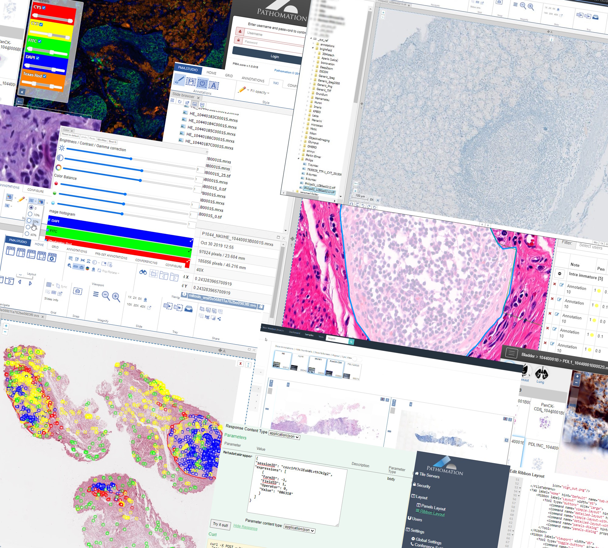
When you say digital pathology or whole slide imaging, sooner or later you end up with OpenSlide. This is essentially a programming library. Back in 2012, a pathologist alerted me to it (there’s some irony to the fact that he found it before me, the bioinformatician). He didn’t know what to do with it, but it looked interesting to him.

OpenSlide is how Pathomation got started. We actually contributed to the project.

We also submitted sample files to add to their public repository (and today, we use this repository frequently ourselves, as do many others, I’m sure).

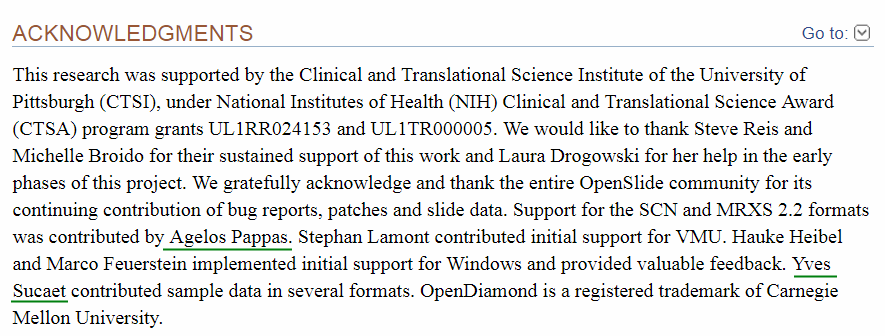
Our names are mentioned in the Acknowledgements section of the OpenSlide paper.

But today, the project has rather slowed down. This is easy to track through their GitHub activity page:

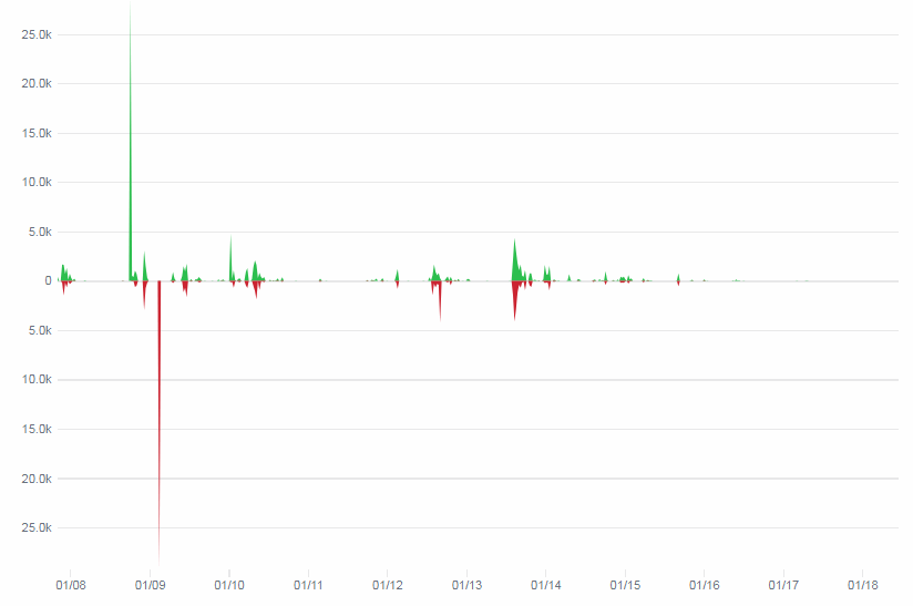
Kudos to the team; they do still make an effort to fix bugs that crop up, today’s but activities seem limited to maintenance. Of course there’s a possibility that nobody gets the code through GitHub anymore, but rather through one of the affiliate projects that they are embedded into.

Consider this though: OpenSlide Discussions about supporting support for (immuno)fluorescence and z-stacking date back to 2012  , but never resulted in anything. Similarly, there are probably about a dozen file formats out there that they don’t support (or flavors that they don’t support, like Sakura’s SVSlide format, which was recently redesigned). We made a table of the formats that we support, and they don’t, at http://free.pathomation.com/pma_start_omero_openslide/

Free at last

Our own software, we’re proud to say, is OpenSlide-free. PMA.start no longer ships with the OpenSlide binaries. The evolution our software has gone through then is as follows (the table doesn’t list all the formats we support; for a full list see http://free.pathomation.com/formats):

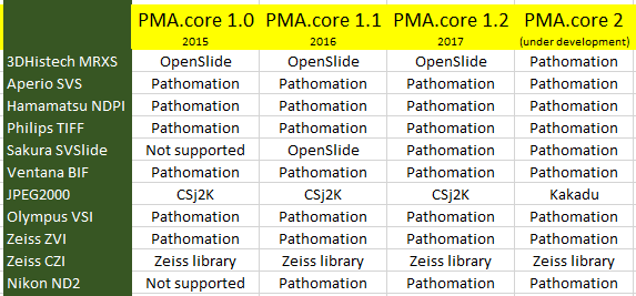
At one time, we realized there was really only one file format left that we still ran through OpenSlide, and with the move to cloud storage (more on that in a later post), we decided we might as well make one final effort to re-implement a parser for 3DHistech MRXS slides ourselves.

Profiling

Of course all of this moving away from OpenSlide is useless if we don’t measure up in terms of performance.

So here’s what we did: we downloaded a number of reference slides from the OpenSlide website. Then, we took our latest GAMP5 validated version of our PMA.core 1.2 software, and rerouted it’s slide parsing routines to OpenSlide. This result in a PMA.core 1.2 build that instead of just 2 (Sakura SVSlide and 3DHistech MRXS), now reads 5 different WSI file formats through OpenSlide:  Sakura SVSlide, 3DHistech MRXS, Leica SCN, Aperio SVS, and Hamamatsu NDPI.

Our test methodology consist of the following steps:

For each slide:
    Determine the deepest zoomlevel
    From this zoomlevel select 200 random tiles
    Retrieve each tile sequentially
    Keep track of how long it takes to retrieve each tiles

We run this scenario of 3 instances of PMA.core:

•                 PMA.core 1.2 without OpenSlide (except for SVSlide and MRXS)
•                 PMA.core 1.2 custom-build with OpenSlide (for all 5 file formats)
•                 PMA.core 2 beta without OpenSlide

The random tiles selected from the respective slides are different each time. The tiles extracted from slide.ext on PMA.core instance 1 are different from the ones retrieved through PMA.core instance 2.

Results

As simple as the above script sounds, we discovered some oddities while running them for each file format.

Let’s start w/ the two easiest to explain ones: SVS and SVSlide.

A histogram of the recorded times for SVSlide yields the following chart:

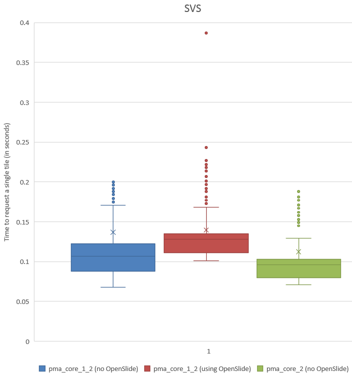
We can see visually that PMA.core 1.2 without OpenSlide is a little faster than the PMA.core 1.2 custom-build with OpenSlide, and that we were able to improve this performance yet again in PMA.core 2.

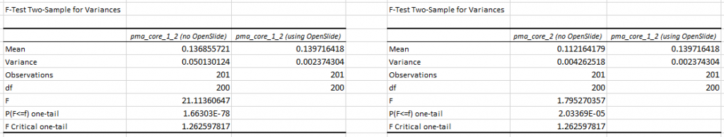
The p-value confirm this. First we do an F-test to determine what T-test we need (p-values of 1.66303E-78 and 2.03369E-05 suggests inequal variances),

Next, we find a p-value of 0.859 (n=200) for the difference in mean tile retrieval time between PMA.core 1.2 with and without OpenSlide, and a p-value of 2.363E-06 for the difference in means between PMA.core 1.2 with OpenSlide and PMA.core 2 without OpenSlide.

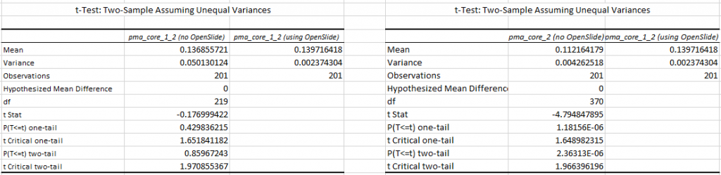
We see this as conclusive evidence that PMA.core 2 (as well as PMA.start, which contains a limited version of the PMA.core 2 code in the form of PMA.core.lite) can render tiles faster than OpenSlide can.

What about SVSlide?

Again, let’s start by looking at the histogram:

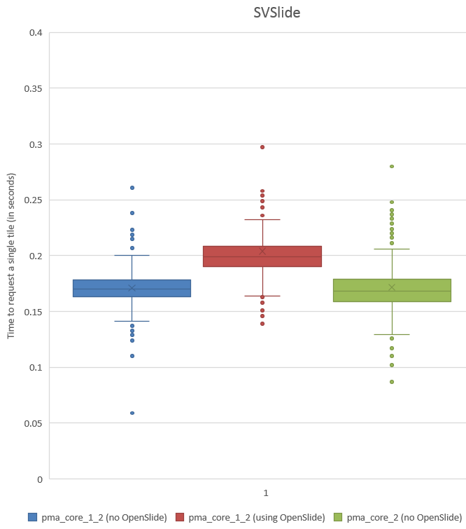
This is the same trend as we saw for SVS, so let’s see if we can confirm this with statistics. The F-statistic between PMA.core 1.2 with and without OpenSlide yields a p-value of 3.064E-22; between PMA.core 1.2 without OpenSlide and PMA.core 2 we get a p-value of 3.068E-13.

Subsequent T-tests (assuming unequal variance) between PMA.core 1.2 with and without OpenSlide show a p-value of  8.031E-19; between PMA.core 1.2 with OpenSlide and PMA.core 2 we get a p-value of 4.10521E-17 (one-tailed).

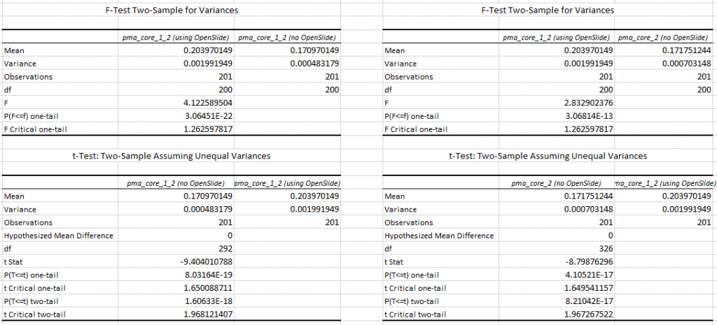
Again, we conclude that both PMA.core 1.2 and PMA.core 2 (as well as PMA.start) are faster to render Sakura SVSlide slides than OpenSlide.

What about the others?

We’re still working on getting data for the other file formats. Stay tuned!

 

 

As mentioned before, I’m the Chief Technology Officer of Pathomation. Pathomation offers a platform of software components for digital pathology. We have a YouTube video that explains the whole thing.

You can try a local desktop-bound (some say “chained”) of our software at http://free.pathomation.com. People tell us our performance is pretty good, which is always nice to hear. The problem is: can we objectively “prove” that we’re fast, too?

The core components of our component suite is aptly called “PMA.core” (we’re developers, not creative namegivers obviously). Conceptually, PMA.core a slide tile server. Simply put, a tile server serves up data in regularised square shaped portions called tiles. In the case of PMA.core, tiles are extracted in real time on an as-needed basis from selected whole slide images.  

So how do you then test tile extraction performance?

At present, I can see three different ways:

1. On a systematic basis, going through all hypothetical tiles one by one, averaging the time it takes to render each one.
2. On a random basis
3. Based on a historical trail of already heavily viewed images.

Each of these methods have their pros and cons, and it depends on what kind of property of the tile server you want to test in the first place.

Systematic testing

The pseudo-code for this one is straightforward:

For x in (0..max_number_of_horizontal_tiles):
  For y in (0..max_number_of_vertical_tiles)
    Extract tile at position (x, y)

However, we’re talking about whole slide image files here, which have more than just horizontal and vertical dimensions. Images are organized as a hierarchical, pyramid-structured stack, and can also contain z-levels, fluorescent layers, or even timelapse data. So the complete loop for systematic testing goes more like this:

For t in (0..max_timeframes):
  For z in (0..max_z_stacks):
    For l in (0..max_zoomlevels):
      For c in (0..max_channels):
        For x in (0..max_number_of_horizontal_tiles):
          For y in (0..max_number_of_vertical_tiles):
            Extract tile at timeframe t, z-stack z, zoomlevel l, channel c, position (x, y)

But that’s just nested looping; nothing fancy about this, really. We’ve been using this method of testing for as long as we can remember pretty much, and even wrapped our own internal tool around this, (again very aptly) called the profiler.

What’s good about this systematic tile test extraction method?

• Easy to understand
• Complete coverage; gives an accurate impression of what effort is needed to re construct the entire slide
• Comparison between file formats (as long as they have similar zoomlevels, z-stacks, channels etc.) allow for benchmarking

What’s bad about this extraction method?

• It’s unrealistic. Users never navigate through a slide tile by tile.
• Considering the ratio of the data being extracted from different dimensions that can occur in a slide, you end up over-sampling some dimensions, while under-sampling others. Again this results in a number that, while accurate, is purely hypothetical, and doesn’t do a good job at illustrating the end-user’s experience.
• In reality, end-users are only presented with a small percentage of the complete “universe” of tiles present in a slide. Ironically, the least interesting tiles will take the smallest amount of effort to send back (especially in terms of bandwidth, like “blank” tiles containing mostly whitespace on a slide or lumens within a specimen etc.)

Random testing

In random testing, we extract a pre-determined (either fixed number or percentage of total number of total available tiles). The pseudo-code is as follows:

Let n = predetermined number of (random) tiles that we want to extract
For i in (0.. n):
  Let t = random (0..max_timeframes)
  Let z = random (0..max_z_stacks)
  Let l = random (0..max_zoomlevels)
  Let c = random (0..max_channels)
  Let x = random (0..max_number_of_horizontal_tiles)
  Let y = random (0..max_number_of_vertical_tiles)
  Extract tile at timeframe t, z-stack z, zoomlevel l, channel c, position (x, y)

The same statistics can be reported back as with systematic testing, in addition to some coverage parameters (based what percentage of total tiles were retrieved).

Let’s look at some of the pros and cons of this one.

Here are the pros:

• Faster than systematic sampling (see also the “one in ten rule” commonly used in statistics: https://en.wikipedia.org/wiki/One_in_ten_rule)
• For deeper zoomlevels that have sufficient data, a more homogenous sampling can be performed (whereas systematic sampling can oversample the deeper zoomlevels, as each deeper zoomlevel contains 4 times more tiles).
• Certain features in the underlying file format (such as storing neighboring tiles close together) that may unjustly boost the results in systematic sampling are less likely to affect results here.

What about the cons?

• Smaller coverage may require bootstrapping to get satisfying aggregate results.
• Random sampling is still unrealistic. Neighboring tiles have less chance of being selected in sequence, while in reality of course any field of view presented to an end-user is the result of compound neighboring tiles
• Less reliable to compare one file format to the next, as this may again require bootstrapping.

Historic re-sampling

A third method can be devised based on historic trace information for one particular file. A file that’s included in a teaching collection and that’s been online for a while, has been viewed by hundreds or even thousands of users. We found in some of our longer running projects (like at http://histology.vub.ac.be or http://pathology.vub.ac.be) that students under such conditions typically are presented with the same tiles over and over again. This means that for a given slide that is fairly often explored, we can reconstruct the order in which the tiles for that particular slide are being served to the end-user, and that trace can be replicated in a testing scenario.

In terms of replication, this is then the most accurate way of testing. Apart from that, other advantages exist:

• This is the best way to measure performance differences across different types of storage media. If for some reason a particular storage medium introduces a performance penalty because of its properties, this is the only reliable way to determine whether that penalty actually matters for whole slide image viewing.
• For large enough numbers (entries in the historical tracing logs), a “natural” mixture of different tiles in different zoomlevels, channels, and z-stacks will be present. This sequence of tiles presented in the trace history automatically reflects how real users navigate a slide.

However, this method, too, has its flaws:

• This type of testing and measuring cannot be used until a slide has actually been online for a certain time period and browsed by a large number of end-users.
• Test results may be affected by the type of user that navigates the slide: we shouldn’t compare historical information about a slide browsed by seasoned pathologists with how novice med school students navigate a different slide. Apples and oranges, you know.
• Because each slide has its own trace, it become really hard to compare performance between different file formats.
• Setting up this type of test requires, of course, historical trace information. This means that this test is the most time consuming to set up: IIS logfiles have to be parsed, tile requests have to be singled out, matched to the right whole slide image etc.

Preliminary conclusions

This section came out of discussing the various strategies with Angelos Pappas, one of our software engineers.

The current profiler that we use was built to do the following:

1. Compare the performance impact of code modifications in PMA.core. For example by changing around a parser class, or by modifying the flow in the core rendering system etc… We needed a way to relatively compare what’s the difference between versions.
2. Compare the performance when rendering different slide formats. To do this, you need similar slides (dimensions, encoding method and of course pixel contents), stored in different formats. The “CMU-{N}” slides from OpenSlide are a good case, as well as the ones we bring back ourselves from various digital pathology events. This again, allows us to do relative comparisons that will give us hints about why a format is slower than another. Is it our parser that needs improvement? Is it the nature of the format? etc.
3. Compare the performance of different storage sources, like local storage versus SMB.

The profiler does all of the above nicely and it’s the only way we have to do such measurements. And even though the profiler supports a “random” mode, we hardly ever use it. Pathomation test engineers usually let the profiler run up to a specific percentage or for a specific period and compare the results.

Eventually what you want to accomplish with all this is to get an objective measurements for user experiences. The profiler wasn’t really meant to measure how good the user experience will be. This is a much more complicated matter, as it involves patterns that are very hard to emulate, network issues, etc etc. For example, if a user zooms into a region, the browser fires simultaneous requests for neighboring tiles. If you ever want to do this kind of measurements, perhaps your best bet would be to do this by commanding a browser. Again though, your measurements would give you a relative comparison.