Angular.JS and PMA.UI

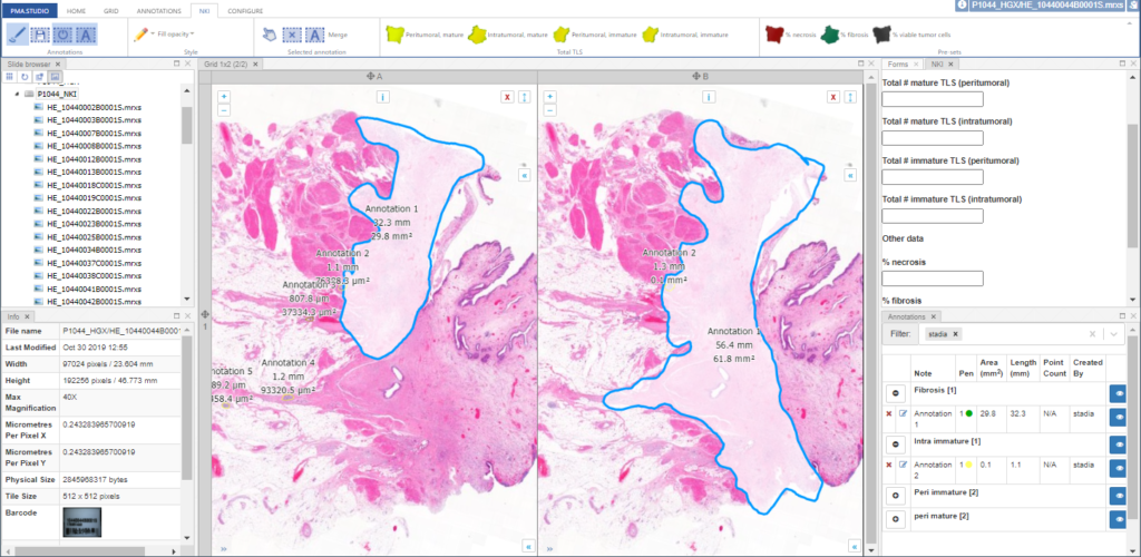
PMA.UI is a Javascript library that provides UI and programmatic components to interact with Pathomation ecosystem. I’s extended interoperability allows it to display WSI slides from PMA.core, PMA.start or Pathomation’s cloud service My Pathomation. PMA.UI can be used in any web app that uses Javascript frameworks (Angular.JS, React.JS etc) or plain HTML webpages.

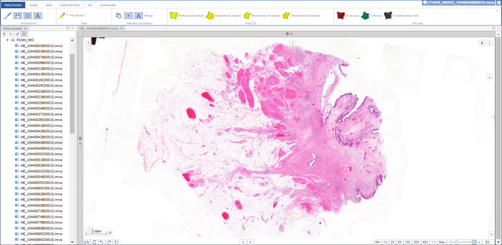
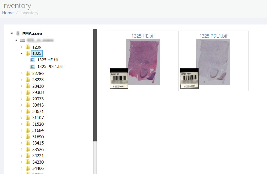
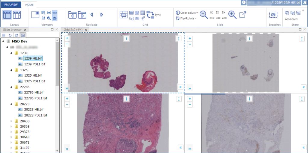
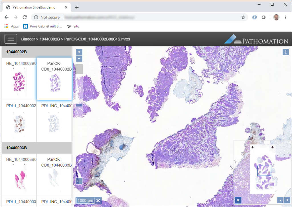
As an example we will use Angular.JS and build an application based on PMA.UI. You can use an existing Angular.JS application or go on and use Angular’s demo application. Our application will have a tree that allows as to view and select directories and slides, a gallery that shows thumbnails of all slides in selected directory, and viewer for displaying selected slide.

First we have to install PMA.UI library using npm by running

npm i @pathomation/pma.ui

inside application’s directory.

Next step is to add JQuery in our app. Open index.html file inside src directory and add

<script src="https://code.jquery.com/jquery-3.3.1.js"
integrity="sha256-2Kok7MbOyxpgUVvAk/HJ2jigOSYS2auK4Pfzbm7uH60="
crossorigin="anonymous">
</script>

after closing body tag. Also we have to add PMA.UI‘s css for components to display correctly. We can do that by opening angular.json file and replace

"styles": [
    "src/styles.css",
],

with

"styles": [
    "src/styles.css",
    "node_modules/@pathomation/pma.ui/dist/pma.ui.css"
],

Now we can start modify PMA.UI component. Delete everything from components html file and add

<div>
    <!-- the element that will host the tree -->
    <div id="tree"></div>

    <!-- the element that will host the gallery -->
    <div id="gallery"></div>

    <!-- the element that will host the viewport -->
    <div id="viewer"></div>
</div>

These are the 3 main components we need. After that add

#tree {
    float: left;
    height: 100%;
    width: 20%;
    max-height: 95vh;
    overflow-y: scroll;
}

#viewer {
    float: left;
    height: 75vh;
    width: 80%;
}

#gallery {
    float: left;
    height: 20%;
    width: 80%;
}

in components css file and change if needed.

It’s time to implement component’s main functionality so open component’s ts file. First of all, we have to import OnInit function from @angular/core and PMA.UI

import { Component, OnInit } from '@angular/core';
import * as PMA from "@pathomation/pma.ui";

and change class to implement OnInit

export class MyComponent implements OnInit {

Lastly we have to create PMA.UI‘s context, slideloader, gallery, and treeview functions and their eventListeners.

ngOnInit() {
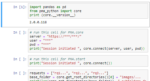
    console.log("PMA.UI version: " + PMA.getVersion());

    // create a context
    var context = new PMA.Context({ caller: caller });

    // add a prompt authentication provider
    new PMA.AutoLogin(context, [{ serverUrl: url, username: username, password: password }]);

    // create an image loader component that will allow us to load images easily
    var slideLoader = new PMA.SlideLoader(context, {
        element: "#viewer",
        overview: {
            collapsed: true
        },
        // the channel selector is only displayed for images that have multiple channels
        channels: {
            collapsed: false
        },
        // the barcode is only displayed if the image actually contains one
        barcode: {
            collapsed: true,
            rotation: 180
        },
        loadingBar: true,
        snapshot: true,
        digitalZoomLevels: 2,
        scaleLine: true,
        filename: true
    });

    // create a tree view that will display the contents of PMA.core servers
    var tree = new PMA.Tree(context, {
        servers: [
            {
                name: "PMA.core",
                url: url,
                showFiles: true
            }
        ],
        element: "#tree",
        preview: true
    });

    // create a gallery that will display the contents of a directory
    var gallery = new PMA.Gallery(context, {
        element: "#gallery",
        thumbnailWidth: 200,
        thumbnailHeight: 140,
        mode: "horizontal",
        showFileName: true
    });

    // listen for the directory selected event by the tree view
    tree.listen(PMA.ComponentEvents.DirectorySelected, function (args) {
        // load the contents of the selected directory
        gallery.loadDirectory(args.serverUrl, args.path);
    });

    // listen for the slide selected event by the tree view
    tree.listen(PMA.ComponentEvents.SlideSelected, function (args) {
        // load the image
        slideLoader.load(args.serverUrl, args.path);
    });

    // listen for the slide selected event to load the selected image when clicked
    gallery.listen(PMA.ComponentEvents.SlideSelected, function (args) {
        // load the image with the context
        slideLoader.load(args.serverUrl, args.path);
    });
}

Build and run your application to check that everything works correctly. That’s it!

You can download complete demo here.

Additional developer resources are provided here.

Customizing the next generation of slide viewer software

It’s coming, it’s coming, it’s coming, it’s coming…

And we’re really excited about it!

We’re in the process of wrapping up PMA.studio. This is going to be our flagship product for the next three years. It’s got everything a microscopy enthusiast needs, ranging from powerful viewport manipulation options, over annotations, to live conferencing. Remember our earlier article about how PMA.core handles (external) slide meta-data? All of that and more is in there, too.

In this blog post, we want to give developers as well as customers in our OEM and reseller program a sneak peek at PMA.studio and specifically focus on the opportunity for custom add-on development and white labeling.

PMA.studio is currently in testing phase for various use cases already, ranging from comparative validation studies to enterprise-wide deployment as a central histological information cockpit. If you are interested in joining the effort and helping us track down last minute bugs, do shoot us an email and we can see if you’re a good fit for our beta-program.

You can find more information about PMA.studio itself in the landing page that we’re building for the software at https://www.pathomation.com/pma.studio.

Administrative console

PMA.studio has a separate interface apart for administrative tasks.

PMA.studio admin console

In the administrative console, you can register any number of PMA.core instances to be used by PMA.studio to retrieve slides from. Once in use, for each registered PMA.core instance, you can see what users have sought access to it.

There’s a general dialog where you can set system-wide settings, like the address to contact in case of trouble, or the company / institute logo to use. This is where white labeling starts.

PMA.studio global settings

Like for PMA.view 1.x, the administrative console in PMA.studio can be used to customize the ribbon interface at top of the interface. The syntax is XML. We don’t have any formal definition of the format, and typically work with customers to get the result they want.

You can play around with the XML code yourself if you want. The default toolbar provides enough example code to allow simple re-arrangements of buttons and move features between different tabs.

PMA.studio ribbon editor

If you run into trouble, there’s always the option to restore the code back to a default toolbar.

Custom annotations

PMA.studio supports annotations. We have a separate tutorial on the subject as part of our beta-program.

There are situations where you don’t want users to go off and make their own annotations at will.

You may want your pathologists to annotate invasive tumor margins or necrotic areas for a study protocol. It’s useful then that people align, and everybody uses the same color scheme. So in addition to providing standard annotation tools, it’s possible to define buttons on your toolbars w/ pre-set attributes and parameters.

Here’s a great example of a project we participated in recently, for which participants had to indicate six different types of tissues / cells:

PMA.studio custom ribbon

The underlaying XML for this extra ribbon tab is as follows:


<Tab label="NKI" hint="custom ribbon tab" name="nki_annotations" enabled="true" visible="true">
    <Ribbon label="Total TLS" width="30%">
        <Tool type="buttons" size="large">
            <Command name="preset-peri_mat" icon="an_m_peri_tls.png" hint="Total # mature TLS (peritumoral)" label="Peritumoral, mature"
                pma-classification="peri mature"
                pma-shape="ClosedFreehand"
                pma-color="#ffff33"
           />
            <Command name="preset-intra_mat" icon="an_m_intra_tls.png" hint="Total # mature TLS (intratumoral)" label="Intratumoral, mature"
                pma-classification="Intra mature"
                pma-shape="ClosedFreehand"
                pma-color="#cccc00"
           />
           <Command name="preset-peri_immat" icon="an_im_peri_tls.png" hint="Total # immature TLS (peritumoral)" label="Peritumoral, immature"
                pma-classification="Peri immature"
                pma-shape="ClosedFreehand"
                pma-color="#999900"
            />
            <Command name="preset-intra_immat" icon="an_im_intra_tls.png" hint="Total # immature TLS (intratumoral)" label="Intratumoral, immature"
                pma-classification="Intra immature"
                pma-shape="ClosedFreehand"
                pma-color="#ffff66"
            />
            </Tool>
        </Ribbon>
        <Ribbon label="Pre-sets" width="30%">
            <Tool type="buttons" size="large">
                <Command name="preset-necrosis" icon="an_necrosis.png" hint="Tumor" label="% necrosis"
                    pma-classification="Necrosis"
                    pma-shape="ClosedFreehand"
                    pma-color="#aa0000"/>
                <Command name="preset-fibrosis" icon="an_macro.png" hint="Tissue" label="% fibrosis"
                    pma-classification="Fibrosis"
                    pma-shape="ClosedFreehand"
                    pma-color="#00aa00"/>
            <Command name="preset-via_tumor" icon="an_tumorcells.png" hint="Tissue" label="% viable tumor cells"
                pma-classification="Viable tumor cells"
                pma-shape="ClosedFreehand"
                pma-color="#000000"/>
        </Tool>
    </Ribbon>
</Tab>

The pay-off of this kind of configuration is two-fold: the protocols are consistently executed as intended. In addition, the training needed for novel users to interact with the software is reduced because they only have a few options to choose from. Less can definitely be more in these scenarios.

Configuring the panel layout

PMA.studio organizes its content across different panels. The layout of PMA.studio is a lot more powerful and flexible than in PMA.view 1.x.

All panels can be turned on or off via the Configuration tab on the ribbon. In addition, the admin console can be used to pre-determine the layout and panel organization when people first log in.

In its simplest configuration, you’re navigating slides and looking at them one by one:

PMA.studio

You can add various information panels as you see fit to get to something that looks more like this:

PMA.studio

Like with the ribbon customization and pre-defined annotation controls, you can pre-set PMA.studio’s panel layout. Again, you’re looking at XML snippets.

The layout from the latter screenshot is then defined as follows:

Iframe panels

A special type of panel is the iframe-panel. With these panels, you can virtually load any website or page that you want within a pre-defined PMA.studio panel. You can define your own panel through the Layout configuration button on the ribbon:

PMA.studio ribbon

A pop-up dialog appears and let’s you specify the title of the panel, and the URL you want it to load.

PMA.studio custom panel

In our example we took  a promotional video for our own PMA.slidebox product (more on that later), but you can put just about anything in there.

The result looks like this:

PMA.studio custom panel

You can pre-define these custom iframe-panels any way you want through the admin console.

<Component name="IFrame" label="Pathomation video" url="https://www.youtube.com/embed/VsiGz8ykuEo"/>

Respective parameters that indicate the current state of the active viewport in PMA.studio are passed along automatically, like this:

http://www.server.com/app/page.php
    ?server=%PATH%TO%PMA%CORE%
    &path=%FULL%PATH%OF%SLIDE%
    &sessionId=%SESSION%ID%

Last but not least: a product pitch

We wrote earlier about PMA.slidebox.

This week, we’ve officially started promoting this product. We updated the landing page for PMA.slidebox, and the first demonstration videos are available through our YouTube channel.

PMA.slidebox

Like with everything we do, we’re very excited about being able to package a ton of useful functionality in nevertheless compact product offering. Do have a look at our demo portal for PMA.slidebox and let us know if this something you, too, are interested in, too!

How to handle slide meta-data?

What is slide meta-data?

In order to know to interact with something, we first need to know what it is. Or, at least, we need you to know what it means for us. Just so we’re clear what we’re talking about.

For the sake of this article, we distinguish three different kinds:

  • Intrinsic meta-data: information stored within a slide’s file format. A trivial example is the slide’s pixel size, and a more advanced feature is the time it took the scanner to produce the slide.
  • User-captured meta-data (forms): Pathomation’s central tile server component, PMA.core, allows for the definition of table structures. Forms are a basic data structure in PMA.core that’s picked up again and used to capture and present user-attributed data in other several Pathomation platform components, including PMA.studio, PMA.slidebox, and PMA.control.
  • External data: if you have tons of external data in a separate repository and want access to it through the Pathomation software platform for digital pathology and virtual microscopy, you can link to it in real-time.

Below you can find an overview of what kind of meta-data is supported by what component and in what capacity

  Slide info Forms External data
PMA.start Read Not supported Not supported
PMA.core Read Define / read Read
PMA.view Read Not supported Not supported
PMA.studio Read Read / write Read
PMA.slidebox Read Read / write Read
PMA.control Read Read / write Read

Slide info

Intrinsic slide meta-data can be shown in PMA.start by clicking on the filename in the viewport.

In the upcoming versions of both PMA.view and PMA.studio, we provide a separate info-panel for this.

There can be more slide info available than is actually shown in our various front-end interfaces. Some information is really specific, too specialized, or irrelevant even to show to most users. Other fields are scanner-specific and don’t make sense to include on a systematic basis.

At the API and SDK level, we provide dedicated SlideInfo calls that return full hierarchical dictionary structures that do give exhaustive slide information and can be consumed as you see fit for your specific application or workflow.

Data with a twist

Forms are defined in PMA.core through the form editor.

PMA.core’s forms support trivial datatypes like text or numbers (of course). We also offer scientifically relevant twists on traditional data capture. An example is that numerical data fields allow the option to be recorded as “below detectable limit”, since it’s very hard to prove that something is not present in a sample. Oftentimes, a numerical zero just means that our detection apparatus just lacks the sensitivity the unmask the presence of a specific phenomenon.

What can you do in forms? Pretty advanced things. We can model the CAP-recommended cancer protocols as PMA.core forms.

PMA.core offers different ways to interact with forms, but it doesn’t provide a data entry module. That’s because it doesn’t really make sense to enter data at this level. Data entry is done in the context of an application or workflow. Our upcoming PMA.studio will support data entry, and PMA.control offers several interaction modes. Underneath, PMA.control interaction modes rely on data stored as PMA.core forms.

You can ask PMA.core to generate a spreadsheet template based on a select folder of slides and a particular already defined form.

At Pathomation, we pride ourselves to be a truly open platform, so PMA.core offers several data formats to export captured form data to, including CSV, XML, and ARFF.

Use cases for external data

Imagine that you organize a toxicology experiment with a rodent population. In a separate database, you’ve been keeping data about each specimen’s vital statistics, dietary and behavior observations, as well as their phenotypic expression and genotypic make-up. Observations happen daily, so that’s 1750 new records per week.

You take weekly biopsies of the animals to monitor their response to a new drug you’re testing. The biopsies are prepared and stained in triplicate (good for a total of 750 new slides per week), and each slide has a barcode that can be used to trace back to the original individual animal. Your slide scanner takes care that the barcode is encoded in the slide’s filename.

Both the slide population and the separate database keep evolving. Replication between your database and a PMA.core form is considered at some point, but deemed inefficient and error-prone, because we are talking about experimental and evolving data structures here.

The solution is to define an external data source in PMA.core. This goes in two steps: first a connection string is defined to connect to the database server.

Next, the external connection is used to formulate any number of queries against.

Data can be previewed within PMA.core, and subsequently is automatically propagated to other environments like PMA.studio.

External data are everywhere. They can be in proprietary databases as in our example above, but they can also be in a (AP)LI(M)S, VNA, PACS, or EHR system. In all those cases, replication is hard and impractical at best, and can even lead to data inconsistencies and errors at worst.

The Pathomation platform for digital pathology and virtual microscopy allows for a more elegant solution.

What WSI data are REALLY made of

Image data types

Pathomation is concerned with any (imaging) data that is microscopy- or pathology-related. Much of the data is large: we talk about gigapixel data, or (more apt for microscopy) whole slide images (WSI).

Not all image data accessed via Pathomation need be large though:

  • Microscopic images can represent individual fields of view, specific areas of interest captured by a mounted camera and for discussion or other ad hoc purposes
  • Pathology starts from physical tissue. Therefore, it is often useful to photograph the obtained tissue. These are typically referred to as “macroscopic images”.

Oftentimes the above results can be stored in common (image) file formats: JPEG and TIFF are most often encountered. You can distribute these images via any medium. But if you have them side by side with your high-resolution images representing prepared slides, it’s reassuring to know that with Pathomation software you can organize these different slides under one umbrella.

Back to the really big data. Elsewhere on this blog, we have an article about the technical challenges when wanting to store an image that contains 100,000 x 200,000 pixels.

We send said article to (potential) customers regularly. Some are helped by it, some not. Because, understandably, many times you just want to know about your slides. When you book a flight, you don’t want to get an explanation about Newton’s or Bernouilli’s laws either… Just get me the tickets please.

So why did we write the article in the first place? Because at Pathomation, we pride ourselves at being format-agnostic. We don’t pick hardware vendors. Each scanner has their pros and cons. Each comes out to server a specific market segment and works better with some tissues than others. It’s not our place to subjectively decide who’s better or worse (although we would appreciate better feedback from some with respect to a vendor’s specific file format).

So please do understand that mentioning specific vendors has nothing to do with any positive or negative endorsements for said vendor. We’re merely stating facts with respect to the way how their techies have long time ago decided to organize their (giga)pixels.

Single or many files

As you already know from the previous article, virtual slides can consist of many different files. Within the files that represent MRXS slides, you find plenty of .dat files, for VSI slides you find .ets files (amongst others) etc.

Several vendors have adopted a single file format for their WSI data. These include Hamamatsu (NDPI), Aperio (SVS), Leica (SCN), and Zeiss (CZI and ZVI).

Other vendors that have adopted a multi-file approach include 3DHistech (MRXS), Olympus (VSI), and Motic (MDS).

The organization of data across multiple files for different vendors is not standardized. In the case of 3DHistech, individual files more or less represent different magnifications. Olympus’ file structure seems more organized around scanned regions of interest.

The single file formats can also be upgraded to multi-file formats. Hamamatsu scanners can create .ndpis files for fluorescent or z-stacked content. The “s” stands for “set”: the .ndpis file merely contains pointers to individual .ndpi files which then each contain the image for the particular layer or channel. You can open these .ndpi files by themselves by the way, but they’re only useful when you also correctly interpret their context from the .ndpis file.

Aperio SVS files can be accompanied by .xml files, which contain annotations. Ventana BIF files can be accompanied by .tifp and .bmp files.

As soon as you have more than 1 file involved, it becomes a multi-file file-format. The strict distinction is important, because some storage systems don’t support multi-file containers.

Examples

Let’s look at the 3DHistech line of scanners: In the screenshot below we scanned two slides: HE and PDL1. The software ends created “HE.mrxs” and “PDL1.mrxs” files, along with “HE” and “PDL1” subfolders.

Within the subfolders, a standard naming convention it used, so you won’t find any more “HE*” files in there.

The .mrxs files themselves are typically just there to allow third-parties to identify these different file-types. Case in point: the .mrxs file can be renamed into a .jpeg file, and then you can just view it as any other image (it’s a quick way for us, too, to display slide thumbnails).

Another example? You got it!

This is what the structure of a .VSI slide looks like:

Each scanned region translates into a “stack”; each stack can contain one or multiple frames.

A different approach, a more hierarchical structure.

For DICOM slides, all related files are grouped together. No subdirectory required:

The details of these for the typical end-user don’t matter, except that they do matter when you want to copy / move/ transfer slides to others. The basic principle here to always make sure you not copy the index .vsi / .mrxs / .whatever file, but also all the accompanying data-files. Zipping them may help both you and your receiving party.

How Pathomation can help

Have a look at our [slides] folder in the Windows Explorer:

Confusing, right?

Now let’s have a look at the same folder through PMA.start eyes:

Since Pathomation knows slides, we systematically hide the intricacies of respective formats that you shouldn’t to worry about. In PMA.start it becomes obvious which subfolders are true subfolders, and which ones are merely there to support vendors’ data structures.

This doesn’t help you yet to transfer slides of course, but if you are one of our commercial users, you typically want to transfer slides from your local system to PMA.core and back. If that is you, then PMA.transfer is a great free tool (it’s part of your license package) for you to look at.

This is how our [slides] folder shows in PMA.transfer:

PMA.transfer seamlessly interfaces with PMA.start, and uses it as a jumping board to transfer slides between different endpoints. The biggest benefit of PMA.transfer therefore is that it encapsulates format-specific complexities and hides them from the end-user. Through PMA.transfer, you’re truly manipulating slides instead of files.

In addition, PMA.transfer also makes sure that only correct slides are transferred (nothing more frustrating than transferring 2 GB of data over Wifi, only to discover that the source was corrupt), as well as confirming that the transfer was completed successfully (probably the second most common source of frustration in the endeavors).

Why it matters

At Pathomation, we take much care designing our components in such a way that data duplication can be avoided at all costs. In PMA.control e.g., you can create as many cases and case collections as you want, but the data always remain in the same location. In PMA.core, you can create nested root-directories, each with different ACL properties. To your end-users these end up looking like different filesystems, but they’re really not. At the API level, we provide the possibility to fingerprint a slide, so you can scan for duplicate files and possibly eliminate them. All of these measures matter when you’re talking about Terabytes of data.

But there comes a time when you do need to copy slides. Perhaps you’re moving them from one installation to another, or there’s a network upgrade, or you just want to ship off some slides to a colleague (My Pathomation can now do this for you, too).

Whatever the case, (virtual) slides will need to be moved around. By their nature, they are big. It helps to have some understanding about how they are structured at that point.

And now you know…

… everything about whole slide images, or, at least, almost everything.

Amongst other things, .mrxs-, .vsi-, and other files help companies like ourselves decide what kind of file format is being used. The alternative would be that we find a large number of subfolders, and we have to parse each and everyone of those folders in a variety of ways to try to “guess” what file format it belongs to (if this is even the case at all; a subfolder can still be a regular subfolder, containing no slides at all). This would be a tremendous drag on system performance.

Whether you deal with Pathomation or another vendor, we hope this article has helped you take a peek behind the curtain of what whole slide images are made of, and how to best work with them.

Of course, if you are using the Pathomation platform, you should have a look at PMA.transfer, a no-hassle tool we developed to facilitate slide transfers.

If you’re not yet a Pathomation customer (whaaaaaaaaaat??), you can contact us for a free no-obligation demonstration.

I “just” want a slide catalog

The case for simplicity

Sometimes user requests are simple. In this particular instance, we had a customer that “just” wanted a list of all of their slides (within a particular root-directory).

We pointed them to the repository of PMA.control:

We pointed them to the tree interface that combines folder and slides in PMA.view:

But as it turned out, these were too complicated. The customer already had built a nested hierarchy of folders and subfolders, but now wanted a linear list of all slides across all folders. A thumbnail next to each slide reference would also be useful, thank you very much.

A linear list of slides

Here’s how we can create a linear list of slides:


from pma_python import core
from datetime import date
from os import mkdir
from os.path import exists

core.connect()

slides = core.get_slides("C:/slides", recursive=True)
print(len(slides), " slides found")     # sanity check

f = open("c:/wsi_report/cat1.html", "w+")
f.write("")
f.write("Market slide catalog created on " + str(date.today()) + "")
f.write("")
for slide in slides:
    f.write(slide + "
") f.write("") f.write("") f.close()

Want to include the thumbnail? Look no further than the get_thumbnail_url method:


f = open("c:/wsi_report/cat2.html", "w+")
f.write("")
f.write("Market slide catalog created on " + str(date.today()) + "")
f.write("")
for slide in slides:
    thumb = core.get_thumbnail_url(slide)
    f.write("" + slide + "
") f.write("") f.write("") f.close()

Ah crap, that looks horrible!

No worries; just add some formatting to the ole’ <img> tag:


f = open("c:/wsi_report/cat3.html", "w+")
f.write("")
f.write("Market slide catalog created on " + str(date.today()) + "")
f.write("")
for slide in slides:
    thumb = core.get_thumbnail_url(slide)
    f.write("" + slide + "
") f.write("") f.write("") f.close()

Yes, something like this:

Much better!

But there’s a catch here: careful observers notice that the thumbnail URLs used by the above code have a PMA.core Session ID embedded. This means that those URLs are only valid as long the respective Session IDs remain valid.

This is fine for ad-hoc reporting, but if we want a list that we can post somewhere on a central server as a reference source for others, we need something just a little more sophisticated. Yes, the keyword in this post is “just”, just in case you’re wondering.

Creating a persistent slide catalog

We want to create a list of all slides in our repository, and we want to list to be persistent. In other words, it is not ok to walk away from our browser for a couple of hours, refresh our list, and see the following:

The solution is to not use the thumbnail URL, but retrieve each thumbnail as a binary object and save it to a subfolder. Then, we let our <img> tag point to the downloaded (or cached, if you will) files.


dir = "c:/wsi_report/cat4/"
if not exists(dir): 
    mkdir(dir)
f = open("c:/wsi_report/cat4.html", "w+")
f.write("")
f.write("Market slide catalog created on " + str(date.today()) + "")
f.write("")
for slide in slides:
    thumb = core.get_thumbnail_image(slide)
    fn = core.get_slide_file_name(slide) + ".jpg"
    thumb_fn = dir + fn
    print("Saving thumbnail as ", thumb_fn)
    thumb.save(thumb_fn)
    f.write("")
    f.write("")
    f.write("" + slide + "
") f.write("") f.write("") f.close()

This catalog fits our needs. We can post it anywhere, and it only relies on local data. You can store it on your hard disk. You don’t need PHP, you don’t need Python, you don’t need the underlying PMA.core (PMA.start in our example code) to be up and running.

There are cons to our approach, too:

  • The catalog takes longer to generate, as we need to download a large number of thumbnails one by one
  • The catalog takes up more space. In our case, for 265 slides, we went from 197 KB to 20+ MB. That’s still manageable to send in a zipped file package, but for larger repositories may become inconvenient.
  • The catalog is a snapshot of the repository. If you use as a reference today and add slides to the underlying root-directory tomorrow, the catalog will not pick up the newly added (or removed, for that matter) slides, unless you re-generate the catalog and re-distribute or publish it.

And finally

Every solution has trade-offs, and even for simple problems, you have think through things to come to the right solution. Problems that have the word “just” somewhere in their formulation can be particularly trickly.

The sourcecode for this post is available through our repository as realdata 038 – simple slide catalog.ipynb. Feel free to download it and adjust it for your own needs.

As always: we encourage interaction. Do let us know what digital pathology problem or scenario you want us to work out in one of our next posts!

My first 6 months @Pathomation

Or the story of me, being thrown to the lions several times.

Digital pathology, a topic I had never heard of six months ago (can you imagine?!) is now one of the most important subjects in my life.

To be honest, I never thought I would have gotten the job at Pathomation, but even though I did not have any experience they still believed in me (or they just gave me the benefit of doubt of course). And for sure I’m glad they did.

I still go to school and before Pathomation, I worked at a local supermarket, which is nice but not very challenging. Now I have to step out of my comfort-zone everyday, doing things I’ve never done and trying to be the best and smartest version of myself, since I’m surrounded by pathologists, scientists etc… Believe me they are a challenge in themselves, but a challenge I’ve accepted happily, because working with people that are so skilled and have such great knowledge is enlightening and motivating.

Step by step and day by day, I’m learning more about medical imaging and the whole world around it. Not only by working from the office, but also abroad. During the first week of January I went to Morocco to work side by side with our Moroccan developers. This was my first work trip ever!

Unfortunately, it was (probably) also the last one of this year, due to unseen circumstances (covid-19, anybody?). I’m waiting for the next trip, even though I’m secretly happy with that little bit of extra time to mentally prepare myself for a medical conference… (which will also be my first one of course)

You might be wondering what I actually do in this company, since I’ve been bragging so much about it in this post. Explaining that in only one paragraph is quite hard, but I’ll try to keep it short.

First of all, I want you to understand, that there’s a variety of things that I actually do, and an array of things that I try to do. All paperwork related things, like bookkeeping, invoicing and preparing estimates, that’s on me! I also try to help Yves by testing our software and giving him my opinion from a user perspective (and hopefully inspire him for new ideas). In actual fact, I try to ease the work of all my colleagues where I can. Because of this, my job contains a wide selection of different tasks, and I’m still exploring what I like to do most.

As you can see, I get lots of chances where I can grow my courage and improve my social skills. Therefore, I’m glad I can be part of this small but growing team!

Optimizing your data volume

Pop quiz

Let’s start this post with a pop-quiz. Without peeking ahead; can you identify what painting it is?

The answer of course is that it’s this one. The question is relevant, because you just proved to yourself that you can get by with very little information to identify something big and important. So let’s just walk you through the way we created the picture above:

  • We took the original image from Wikipedia, provided through the WikiMedia Commons library, at 585 x 870 pixels (a total of 508,950 pixels). The physical size of this image was 957 KB.
  • We then resized this image to thumbnail size of 27 x 40 pixels (a total of 1,080 pixels, or a reduction by 99.8%). The physical size of this image was around 3 KB (a reduction by 99.7%).
  • We then blew up the thumbnail again with a factor 10 to 270 x 400 pixels (bringing the total amount of pixels again to 108,000 or about 21% of the original). Interestingly enough, the image size this time is 75 KB, which represents only about 8% (even though we supposedly offer 21% of the original pixels).

The important takeaway is that the human brain is remarkable in filtering out and handling noisy, blurry data.

But what does this have to do with digital pathology or virtual microscopy?

A bottleneck

Recently we were contacted by a company that was involved in telepathology in rather rural areas. It’s a great endeavor: they provide local staff with refurbished scanners, thereby hoping to extend advanced pathology expertise to communities that have no other way of having access to these.

But as anybody working with whole slide images can attest: they’re big. Huge sometimes, And there’s no way around this. And it’s a problem for our contact because rural areas unfortunately oftentimes also still mean limited bandwidth. It can take hours to transfer a single slide, and that’s just not practical.

This is where our earlier exercise comes into play. And the question now becomes: How much information do you really need to make an accurate diagnosis?

If we scan a slide at 40X (0.25 ppm according to DICOM’s definition) and we brought it back down to 20X (0.5 ppm), would it be sufficient for a pathologist to make an accurate diagnosis? And what about image compression? Do we need 100%? What if we transferred the image with 90% quality? 80%? We know that at 50% compression artifacts will not result in a pretty image, but the real question is whether the receiving pathologist can still make a diagnosis.

Some research has done on this: Yukako et al concluded that even significant compression ratios have no impact on diagnostic accuracy.

So with that being said, how could you do it? And how would you do it with the Pathomation platform?

To Jupyter, capt’n!

A whole slide image has two properties that we can manipulate to control the physical slide size:

  • The highest zoomlevel contained in the slide (see also our blog post of WSI structure)
  • The compression ratio of individual tissue tiles

We can then create a jupyter script can takes in these two parameters, to convert any given slide to an intermediate format. We choose TIFF here, but you can adapt the output to your own needs.

The first one is target-quality, and can be given a value of 0-100 (100 being the highest quality).

The second one is the downscale factor. It can be chosen from a list of values of [1, 2, 4, 8, 16, 32, 64, 128]. That doesn’t quite translate to an optical magnification or pixels per micron reading, but we use it here for the sake of simplicity (it has to do with the way these WSI data are typically structured). The higher the downscale factor, the less magnification and detail you will end up with. If you want to, you can write your own conversion method from downscale-factor to ppm and back again.

After setting the parameters, we create new TIFF file using the GDAL TIFF driver. The width and height of the final tiff is based on number of tiles horizontally and vertically.

We read each tile of the final zoomlevel (1:1 resolution) from the server and write it to the resulting TIFF file Then we create the pyramid of the file using BuildOverviews function of GDAL

The complete Jupyter notebook is available from our website.

The jury is in session

Let’s see what the result of our code is for different combinations.

We downloaded CMU-1.svs from the OpenSlide sample data repository, which has a compression quality of 30%. The original file size is 169 MB.

When we run our script and ask to generate a derived TIFF slides with 100% tile quality and the same magnification level, we find something interesting: the new slide is about 1.5 GB is slide. It became bigger!

This is our first lesson then: when doing these kind of conversions, it doesn’t make any sense to transfer data at a compression rate that’s lower than the original slide’s compression.

The CMU-1.svs slide is an extreme case. We haven’t heard of any labs that are scanning at only 30% quality; most scanners are usually calibrated to produce data at 70%-80% compression quality.

That being said, let’s just use the 1.5 GB as a reference point and see how the data package becomes smaller as we vary both the compression quality and the downsampling parameter:

Not surprisingly, as the scaling factor goes up (a scaling factor of 4 would roughly correspond with a perceived magnification of 10X), the resulting slide size becomes significantly smaller.

So in both axes, significant saving are to be had. Similar to the Mona Lisa painting example that we started with; the slide at 10X and 60% quality is only 2.3% the filesize of the original 40X and 100% quality file.

What else?

We wrote this article to give you ideas on how you can employ PMA.start to optimize your data volume when shuttling back data back and forth between two sites.

This is but one scenario to consider. Is the eventual resolution sufficient to maintain diagnostic accuracy? That’s up to you and your pathologist(s) to resolve. Whether the parameters specified here work for you, is a question you can only answer.

To give you an idea; here’s the slide with a downsampling rate of 1, and 100% compression quality:

Here’s the same slide with a downsampling rate of 4, and only 60% compression quality:

There is one more interesting experiment to consider here: storage for digital pathology doesn’t scale very well, and we would be interested to see whether machine learning algorithms (ML/DL/AI) could be trained equally well on heavily compressed data, compared to uncompressed data.

Full disclosure here: There are things missing here, too. We’re not incorporating the thumbnail image in the exported TIFF, in similar fashion as certain other vendors do this. It’s possible, but again, the eventual implementation depends on your personal preference and circumstances. If you’re looking for help and advice with this, we can assist you and you may contact us at slides@pathomation.com.

More business intelligence

The story of the three Qs

In this article, we explain how Pathomation was recently able to assist its one of its customers with Performance Qualification tests for a new slide scanner.

At our customer’s lab, each piece of equipment that they take into operation, goes through a rigorous qualification pipeline before putting it to work for day-to-day lab activities.

This goes for slide scanners as well.

The qualification pipeline (the “validation procedure”) consists of three steps:

  • Installation Qualification (IQ)
  • Operational Qualification (OQ)
  • Performance Qualification (PQ)

The first step is straightforward: you’re asking yourself if the scanner can scan your slides or not. Is the type of glass slide that your lab use, in combination with the coverslip, compatible with the new scanner? Is the barcode on the slide label scanned properly, too? What about (automated) tissue detection?…

The second step is operational qualification: can the new equipment handle the edge parameters of your day-to-day operations? If you plan to feed the scanner up to 400 slides per day; will that work?

The third step in the validation can be somewhat subjective, and it’s here that Pathomation’s software platform came in particularly handy.

Performance Qualification

Performance Qualification (PQ) is a test procedure that takes place in order to verify if a new piece of equipment is good enough to be put to work in the daily workflow of a company. It happens after the hardware has already gone through IQ and OQ.

Our customer recently wanted to know how their various scanners compare to a new one in terms of speed. They took a representative set of slides, divided it in three groups (“requests”), and then put each scanner to work.

their various scanners compare to a new one in terms of speed. They took a representative set of slides, divided it in three groups (“requests”), and then put each scanner to work.

In the vendor’s viewer software, one of the parameters that could be seen was “scanning duration”. Considering the side of the dataset however, opening each slide individually in the viewer software, noting down the scanning time, recording it into an Excel sheet etc., would have been a very tedious task.

So they turned to Pathomation for help: Can Pathomation’s software be used to create a table with all scan duration values for all scanned slides?

Our API

Pathomation’s API offers a get_slide_info() call. We used it in our first article on business intelligence to extract specific bits of information with it. The method be default returns a nested hierarchy of information.

But not every scanner exports the same information. Some of the slide information we expose ourselves through ImageInfo, some not. This is because vendor 1 exposes (A, B, C, D, E), vendor 2 exposes (A, B, F, G, H), vendor 3 exposes (A, B, C, I, J, K, L) etc. Therefore, Pathomation offers the common denominator information only, something like (A, B, C).

In order to maintain some standardization across the different vendors, part of the returned information by get_slide_info is a MetaData array that contains key-value pairs that may or may not be provided by your scanner vendor.

As it turns out, we didn’t have the scanning time in there yet, but because of the already provided structure, it was straightforward to add it.

Like our first business intelligence exercise, we then write a wrapper method to extract the scanning duration as we need it:

def get_scanning_duration(slide_ref):
    info = core.get_slide_info(slide)
    meta = info["MetaData"]
    for meta_el in meta:
        if (meta_el["Name"] == "ScanningDuration"):
            return meta_el["Value"]
    return -1

The remainder of the script is straightforward:

  • Loop over the different scanner output
    • Foreach scanner (“request”), get all the slides (recursively in our case)
      • Foreach slide, extract the scanning duration
  • Wrap all output into a Pandas dataframe structure
  • Export the Dataframe to a spreadsheet

A word about that last step. On occasion, people have called us old-fashioned for this one. Surely Excel is spread wide and far enough by now so that it can be considered a de facto “standard” file format, too, can’t it?

I disagree. I still prefer to use csv instead of Excel. Why? Because csv files are simple, and transportable to many other platforms and applications. Our data in this case consists of a single table with three columns. It’s simple. We don’t need a complex data format to store this kind of data.

Generating fancy file format output is not part of the assignment here. Keep It Simple.

Our final code looks like this and can be downloaded as a Jupyter notebook, so you can play around with it yourself.


server = "http://***/***"
user = "***"
pwd = "***"
print("Session initiated ", core.connect(server, user, pwd))
requests = ["RQ105", "RQ204", "RQ695"]
base_folder = " Images/pq"
print(len(core.get_directories(base_folder)), " subfolders detected in root base folder", base_folder)
s_times = []
for req in requests:
    print(base_folder + "/" + req)
    for slide in core.get_slides(base_folder + "/" + req, recursive=True):
        s_times.append({"slide": str(slide).replace(base_folder, ""), "scan_time": get_scanning_duration(slide), "request": str(req)})
scan_times = pd.DataFrame(s_times, columns=["request", "slide", "scan_time"])
scan_times.to_csv("scanning duration.csv")

What about the results?

We can import the resulting CSV file in Excel and see what it looks like:

As we’re interested in comparing the different scanners to one another, one direct way to do this is with a pivot-chart.

These are the results. What do you think? Do all three scanners perform equally? Does the new scanner pass performance qualification (PQ)?

Your challenge here

This is how Pathomation works with its customers.

Our philosophy has been and remains to develop local, and then scale as you handle more complex scenarios. You do not need the commercial version of PMA.core to get to work with the code in this post. The Jupyter notebook that comes with this blog post is suited for use for both PMA.start and PMA.core.

Do you use Pathomation software in your daily workflows already? Tell us your business intelligence challenge and perhaps we’ll address is in an upcoming post!

A look at PMA.slidebox

So what if you “just” want to show your slides?

Education is one of the main application domains of digital pathology. And there are many instances where you just have a couple of slides that you want people to look at. When Pathomation first became involved in deploying its software for facilitating seminars, we used PMA.view.

But while it’s possible to do this, PMA.view is not a good solution for this particular problem:

  • People still need to login in PMA.view
  • PMA.view requires telling people where to navigate to (which root-directories / paths); your root-directories on the PMA.core side of things may not exactly reflect the content that you want people to see.
  • PMA.core is folder-based navigation, and PMA.view is too. This means that the concept of a case (a group of slides belonging to a patient or experiment) is not intuitively represented
  • neither PMA.view nor PMA.core support any of the visual cue-elements that we’ve all gotten accustomed to in recent years such as avatars.
  • The learning curve of PMA.view is still too steep for people that just need to look at slides. PMA.view is overshooting for what you want people to actually experience

How did people used to do it? They traveled to conferences with a slidebox in their hand luggage. Within the slidebox; neatly organized slides, sorted by case. We don’t want to be sensational here and say that the slides got lost all the same, or that they broke all the time, or got confiscated by security in a post-9/11 world (glass slides + ninja pathologist = impromptu shiroken?).

But: things could happen when traveling with physical slides, and the most likely issue was probably still somebody forgetting to take their slides with them in the first place!

Also: when traveling with physical slides you depend heavily on the organization’s talent of providing and calibrating multi-headed microscope equipment. As more people attend, aligning all the optics of these becomes ever harder, and for large groups this is just impractical.

Cue PMA.slidebox

So we got thinking… If people are used to physical slideboxes, why not just make a virtual slidebox? This is exactly what PMA.slidebox is and does!

PMA.slidebox, like all our software, relies on PMA.core. It means that you can use all the great features of PMA.core (different root-directories, access control), without having to explain it to your audience.

All your audience sees, without to register or login or need to install or download anything (zero footprint) is this:

So how does it work? PMA.slidebox shows up to four collections in the top-left corner of the screen (screenshot only shows three). When you select a collection, you see the “cases” appear underneath it, along with the slides for each “case”.

We put the word “case” between quotes deliberately because you don’t have to set it up this way. You can have a simple list of slides without any hierarchy or structure to it, and PMA.slidebox will pick it up. Similarly, if you only have a couple of cases, you could turn those into individual collections, and present them as such.

What you want to show and how you want to show it is completely up to you. It’s just like a real slidebox: you put the slides in that you want, and you organize them the way you want them, too.

Want to give it a go yourself? Here’s an example how such a virtual slidebox works in practice: http://host.pathomation.com/p0022_slidebox/

Configuration

PMA.slidebox is flexible. It is hosted on a website, somewhere (can be on your infrastructure, or on ours). If you don’t have PHP, we can configure it for you; but if you do, you can configure everything by yourself via a configuration panel.

What you first need to do is decide how you want to have everything structured. You can build a hierarchy of up to three deep, with the following levels:

As you have only 4 cases in the above screenshot, you could simplify your hierarchy like this:

While PMA.slidebox is flexible, we should point out that it is necessary to have some kind of hierarchy at least. You cannot just dump all your slides into a single folder and expect the software to figure it out from there.

Note: if you do have large repositories of slides, and you want structured case creation and organization, you should have a look at PMA.control.

Here’s what the setup looks like when your spread your cases across only two collections:

And here’s what that same group of slides looks like, but this time with each case being defined as its own separate collection:

In closing

With our PMA.slidebox product, Pathomation solves the problem of mass-distribution of slide collections. When you just want to share your slides with people in a somewhat organized (collection and cases) fashion, PMA.slidebox is the perfect solution for you. The easy to use configuration panel behind the front-end makes it a breeze to point to the exact content that you want to display, and under no circumstances does the end-user have to do anything else except click on the URL that you provide them with.

Find out more about PMA.slidebox at our website at http://www.pathomation.com/pma-slidebox.

Pathomation on the web

Web presence

We want talk a bit more about our different communication channels this week.

When you’re reading this article, you’ve obviously found one of them.

The RealData blog at http://realdata.pathomation.com is a wordpress website that we set up a couple of years ago to allow us to communicate about or explain topics that don’t necessarily have a dedicated place yet on our “main” company website at http://www.pathomation.com.

Pathomation is a small company, and things can move quickly. We simply don’t have time to re-do our website each month or so because our product offering changes, or because there’s a spurt in creative writing that needs to find a landing spot and reach an audience. A free-form blog then seemed like a good idea.

And we still think it is 😊

There are companies whose website is a blog, but we do think there’s still a need to offer structured information and a general product overview as well.

So while you can’t constantly rewrite your website, we did manage to re-work http://www.pathomation.com this month and we’re pretty proud of the result. If you haven’t checked it out yet, go ahead and do so. It’s a lot more comprehensive than anything we’ve had up before.

And if you’ve read this blog, of course you’ve heard about PMA.start before, our free whole slide image / digital pathology viewer software that can be used by anybody for anything to manage their local slide content. Our http://free.pathomation.com website is the third axis of our online web-presence strategy.

PMA.start comes with no limitations, except the one that is built-in: you can only use it on local content. If you want to share data with colleagues via a network, you need to upgrade to our professional PMA.core product. If you’re not quite sure what that’s all about, you can still sign up for our beta program until the end of this month (just a few days left, so be quick).

Check out our beta landing page at https://www.pathomation.com/beta

And there you have it; our three pronged strategy to provide you, our valued customer and end-user, with background information about the Pathomation universe, and our great products.